目录
导言
导入和设置
准备数据集
实施多层感知器(MLP)
实施补丁创建层
显示输入图像的补丁
实施补丁编码层
构建 ViT 模型
运行实验
评估模型
政安晨的个人主页:政安晨
欢迎 👍点赞✍评论⭐收藏
收录专栏: TensorFlow与Keras机器学习实战
希望政安晨的博客能够对您有所裨益,如有不足之处,欢迎在评论区提出指正!
本文目标:使用视觉变换器进行物体检测的简单 Keras 实现。
导言
Alexey Dosovitskiy 等人撰写的文章 Vision Transformer (ViT) 架构表明,直接应用于图像片段序列的纯变换器可以很好地完成物体检测任务。
在本 Keras 示例中,我们实现了对象检测 ViT,并在 Caltech 101 数据集上对其进行训练,以检测给定图像中的飞机。
导入和设置
import os

os.environ["KERAS_BACKEND"] = "jax"  # @param ["tensorflow", "jax", "torch"]


import numpy as np
import keras
from keras import layers
from keras import ops
import matplotlib.pyplot as plt
import numpy as np
import cv2
import os
import scipy.io
import shutil
准备数据集
我们使用加州理工学院 101 数据集。
# Path to images and annotations
path_images = "./101_ObjectCategories/airplanes/"
path_annot = "./Annotations/Airplanes_Side_2/"

path_to_downloaded_file = keras.utils.get_file(
    fname="caltech_101_zipped",
    origin="https://data.caltech.edu/records/mzrjq-6wc02/files/caltech-101.zip",
    extract=True,
    archive_format="zip",  # downloaded file format
    cache_dir="/",  # cache and extract in current directory
)
download_base_dir = os.path.dirname(path_to_downloaded_file)

# Extracting tar files found inside main zip file
shutil.unpack_archive(
    os.path.join(download_base_dir, "caltech-101", "101_ObjectCategories.tar.gz"), "."
)
shutil.unpack_archive(
    os.path.join(download_base_dir, "caltech-101", "Annotations.tar"), "."
)

# list of paths to images and annotations
image_paths = [
    f for f in os.listdir(path_images) if os.path.isfile(os.path.join(path_images, f))
]
annot_paths = [
    f for f in os.listdir(path_annot) if os.path.isfile(os.path.join(path_annot, f))
]

image_paths.sort()
annot_paths.sort()

image_size = 224  # resize input images to this size

images, targets = [], []

# loop over the annotations and images, preprocess them and store in lists
for i in range(0, len(annot_paths)):
    # Access bounding box coordinates
    annot = scipy.io.loadmat(path_annot + annot_paths[i])["box_coord"][0]

    top_left_x, top_left_y = annot[2], annot[0]
    bottom_right_x, bottom_right_y = annot[3], annot[1]

    image = keras.utils.load_img(
        path_images + image_paths[i],
    )
    (w, h) = image.size[:2]

    # resize images
    image = image.resize((image_size, image_size))

    # convert image to array and append to list
    images.append(keras.utils.img_to_array(image))

    # apply relative scaling to bounding boxes as per given image and append to list
    targets.append(
        (
            float(top_left_x) / w,
            float(top_left_y) / h,
            float(bottom_right_x) / w,
            float(bottom_right_y) / h,
        )
    )

# Convert the list to numpy array, split to train and test dataset
(x_train), (y_train) = (
    np.asarray(images[: int(len(images) * 0.8)]),
    np.asarray(targets[: int(len(targets) * 0.8)]),
)
(x_test), (y_test) = (
    np.asarray(images[int(len(images) * 0.8) :]),
    np.asarray(targets[int(len(targets) * 0.8) :]),
)
实施多层感知器(MLP)
我们使用 Keras 示例 "使用视觉转换器进行图像分类 "中的代码作为参考。
def mlp(x, hidden_units, dropout_rate):
    for units in hidden_units:
        x = layers.Dense(units, activation=keras.activations.gelu)(x)
        x = layers.Dropout(dropout_rate)(x)
    return x
实施补丁创建层
class Patches(layers.Layer):
    def __init__(self, patch_size):
        super().__init__()
        self.patch_size = patch_size

    def call(self, images):
        input_shape = ops.shape(images)
        batch_size = input_shape[0]
        height = input_shape[1]
        width = input_shape[2]
        channels = input_shape[3]
        num_patches_h = height // self.patch_size
        num_patches_w = width // self.patch_size
        patches = keras.ops.image.extract_patches(images, size=self.patch_size)
        patches = ops.reshape(
            patches,
            (
                batch_size,
                num_patches_h * num_patches_w,
                self.patch_size * self.patch_size * channels,
            ),
        )
        return patches

    def get_config(self):
        config = super().get_config()
        config.update({"patch_size": self.patch_size})
        return config
显示输入图像的补丁
patch_size = 32  # Size of the patches to be extracted from the input images

plt.figure(figsize=(4, 4))
plt.imshow(x_train[0].astype("uint8"))
plt.axis("off")

patches = Patches(patch_size)(np.expand_dims(x_train[0], axis=0))
print(f"Image size: {image_size} X {image_size}")
print(f"Patch size: {patch_size} X {patch_size}")
print(f"{patches.shape[1]} patches per image \n{patches.shape[-1]} elements per patch")


n = int(np.sqrt(patches.shape[1]))
plt.figure(figsize=(4, 4))
for i, patch in enumerate(patches[0]):
    ax = plt.subplot(n, n, i + 1)
    patch_img = ops.reshape(patch, (patch_size, patch_size, 3))
    plt.imshow(ops.convert_to_numpy(patch_img).astype("uint8"))
    plt.axis("off")
演绎展示:
Image size: 224 X 224
Patch size: 32 X 32
49 patches per image
3072 elements per patch

实施补丁编码层
PatchEncoder 层通过将补丁投影到大小为 projection_dim 的矢量中,对补丁进行线性变换。它还会在投影向量中添加可学习的位置嵌入。
class PatchEncoder(layers.Layer):
    def __init__(self, num_patches, projection_dim):
        super().__init__()
        self.num_patches = num_patches
        self.projection = layers.Dense(units=projection_dim)
        self.position_embedding = layers.Embedding(
            input_dim=num_patches, output_dim=projection_dim
        )

    # Override function to avoid error while saving model
    def get_config(self):
        config = super().get_config().copy()
        config.update(
            {
                "input_shape": input_shape,
                "patch_size": patch_size,
                "num_patches": num_patches,
                "projection_dim": projection_dim,
                "num_heads": num_heads,
                "transformer_units": transformer_units,
                "transformer_layers": transformer_layers,
                "mlp_head_units": mlp_head_units,
            }
        )
        return config

    def call(self, patch):
        positions = ops.expand_dims(
            ops.arange(start=0, stop=self.num_patches, step=1), axis=0
        )
        projected_patches = self.projection(patch)
        encoded = projected_patches + self.position_embedding(positions)
        return encoded
构建 ViT 模型
ViT 模型有多个变换器模块。
多头注意层(MultiHeadAttention)用于自注意,应用于图像补丁序列。编码补丁(跳过连接)和自我注意层的输出被归一化,并输入多层感知器(MLP)。
该模型输出代表物体边界框坐标的四个维度。
def create_vit_object_detector(
    input_shape,
    patch_size,
    num_patches,
    projection_dim,
    num_heads,
    transformer_units,
    transformer_layers,
    mlp_head_units,
):
    inputs = keras.Input(shape=input_shape)
    # Create patches
    patches = Patches(patch_size)(inputs)
    # Encode patches
    encoded_patches = PatchEncoder(num_patches, projection_dim)(patches)

    # Create multiple layers of the Transformer block.
    for _ in range(transformer_layers):
        # Layer normalization 1.
        x1 = layers.LayerNormalization(epsilon=1e-6)(encoded_patches)
        # Create a multi-head attention layer.
        attention_output = layers.MultiHeadAttention(
            num_heads=num_heads, key_dim=projection_dim, dropout=0.1
        )(x1, x1)
        # Skip connection 1.
        x2 = layers.Add()([attention_output, encoded_patches])
        # Layer normalization 2.
        x3 = layers.LayerNormalization(epsilon=1e-6)(x2)
        # MLP
        x3 = mlp(x3, hidden_units=transformer_units, dropout_rate=0.1)
        # Skip connection 2.
        encoded_patches = layers.Add()([x3, x2])

    # Create a [batch_size, projection_dim] tensor.
    representation = layers.LayerNormalization(epsilon=1e-6)(encoded_patches)
    representation = layers.Flatten()(representation)
    representation = layers.Dropout(0.3)(representation)
    # Add MLP.
    features = mlp(representation, hidden_units=mlp_head_units, dropout_rate=0.3)

    bounding_box = layers.Dense(4)(
        features
    )  # Final four neurons that output bounding box

    # return Keras model.
    return keras.Model(inputs=inputs, outputs=bounding_box)
运行实验
def run_experiment(model, learning_rate, weight_decay, batch_size, num_epochs):
    optimizer = keras.optimizers.AdamW(
        learning_rate=learning_rate, weight_decay=weight_decay
    )

    # Compile model.
    model.compile(optimizer=optimizer, loss=keras.losses.MeanSquaredError())

    checkpoint_filepath = "vit_object_detector.weights.h5"
    checkpoint_callback = keras.callbacks.ModelCheckpoint(
        checkpoint_filepath,
        monitor="val_loss",
        save_best_only=True,
        save_weights_only=True,
    )

    history = model.fit(
        x=x_train,
        y=y_train,
        batch_size=batch_size,
        epochs=num_epochs,
        validation_split=0.1,
        callbacks=[
            checkpoint_callback,
            keras.callbacks.EarlyStopping(monitor="val_loss", patience=10),
        ],
    )

    return history


input_shape = (image_size, image_size, 3)  # input image shape
learning_rate = 0.001
weight_decay = 0.0001
batch_size = 32
num_epochs = 100
num_patches = (image_size // patch_size) ** 2
projection_dim = 64
num_heads = 4
# Size of the transformer layers
transformer_units = [
    projection_dim * 2,
    projection_dim,
]
transformer_layers = 4
mlp_head_units = [2048, 1024, 512, 64, 32]  # Size of the dense layers


history = []
num_patches = (image_size // patch_size) ** 2

vit_object_detector = create_vit_object_detector(
    input_shape,
    patch_size,
    num_patches,
    projection_dim,
    num_heads,
    transformer_units,
    transformer_layers,
    mlp_head_units,
)

# Train model
history = run_experiment(
    vit_object_detector, learning_rate, weight_decay, batch_size, num_epochs
)


def plot_history(item):
    plt.plot(history.history[item], label=item)
    plt.plot(history.history["val_" + item], label="val_" + item)
    plt.xlabel("Epochs")
    plt.ylabel(item)
    plt.title("Train and Validation {} Over Epochs".format(item), fontsize=14)
    plt.legend()
    plt.grid()
    plt.show()


plot_history("loss")
演绎展示:
Epoch 1/100
 18/18 ━━━━━━━━━━━━━━━━━━━━ 9s 109ms/step - loss: 1.2097 - val_loss: 0.3468
Epoch 2/100
 18/18 ━━━━━━━━━━━━━━━━━━━━ 0s 25ms/step - loss: 0.4260 - val_loss: 0.3102
Epoch 3/100
 18/18 ━━━━━━━━━━━━━━━━━━━━ 0s 25ms/step - loss: 0.3268 - val_loss: 0.2727
Epoch 4/100
 18/18 ━━━━━━━━━━━━━━━━━━━━ 0s 25ms/step - loss: 0.2815 - val_loss: 0.2391
Epoch 5/100
 18/18 ━━━━━━━━━━━━━━━━━━━━ 0s 25ms/step - loss: 0.2290 - val_loss: 0.1735
Epoch 6/100
 18/18 ━━━━━━━━━━━━━━━━━━━━ 0s 24ms/step - loss: 0.1870 - val_loss: 0.1055
Epoch 7/100
 18/18 ━━━━━━━━━━━━━━━━━━━━ 0s 25ms/step - loss: 0.1401 - val_loss: 0.0610
Epoch 8/100
 18/18 ━━━━━━━━━━━━━━━━━━━━ 0s 25ms/step - loss: 0.1122 - val_loss: 0.0274
Epoch 9/100
 18/18 ━━━━━━━━━━━━━━━━━━━━ 0s 8ms/step - loss: 0.0924 - val_loss: 0.0296
Epoch 10/100
 18/18 ━━━━━━━━━━━━━━━━━━━━ 0s 24ms/step - loss: 0.0765 - val_loss: 0.0139
Epoch 11/100
 18/18 ━━━━━━━━━━━━━━━━━━━━ 0s 25ms/step - loss: 0.0597 - val_loss: 0.0111
Epoch 12/100
 18/18 ━━━━━━━━━━━━━━━━━━━━ 0s 25ms/step - loss: 0.0540 - val_loss: 0.0101
Epoch 13/100
 18/18 ━━━━━━━━━━━━━━━━━━━━ 0s 24ms/step - loss: 0.0432 - val_loss: 0.0053
Epoch 14/100
 18/18 ━━━━━━━━━━━━━━━━━━━━ 0s 24ms/step - loss: 0.0380 - val_loss: 0.0052
Epoch 15/100
 18/18 ━━━━━━━━━━━━━━━━━━━━ 0s 25ms/step - loss: 0.0334 - val_loss: 0.0030
Epoch 16/100
 18/18 ━━━━━━━━━━━━━━━━━━━━ 0s 25ms/step - loss: 0.0283 - val_loss: 0.0021
Epoch 17/100
 18/18 ━━━━━━━━━━━━━━━━━━━━ 0s 24ms/step - loss: 0.0228 - val_loss: 0.0012
Epoch 18/100
 18/18 ━━━━━━━━━━━━━━━━━━━━ 0s 8ms/step - loss: 0.0244 - val_loss: 0.0017
Epoch 19/100
 18/18 ━━━━━━━━━━━━━━━━━━━━ 0s 8ms/step - loss: 0.0195 - val_loss: 0.0016
Epoch 20/100
 18/18 ━━━━━━━━━━━━━━━━━━━━ 0s 8ms/step - loss: 0.0189 - val_loss: 0.0020
Epoch 21/100
 18/18 ━━━━━━━━━━━━━━━━━━━━ 0s 8ms/step - loss: 0.0191 - val_loss: 0.0019
Epoch 22/100
 18/18 ━━━━━━━━━━━━━━━━━━━━ 0s 8ms/step - loss: 0.0174 - val_loss: 0.0016
Epoch 23/100
 18/18 ━━━━━━━━━━━━━━━━━━━━ 0s 8ms/step - loss: 0.0157 - val_loss: 0.0020
Epoch 24/100
 18/18 ━━━━━━━━━━━━━━━━━━━━ 0s 8ms/step - loss: 0.0157 - val_loss: 0.0015
Epoch 25/100
 18/18 ━━━━━━━━━━━━━━━━━━━━ 0s 8ms/step - loss: 0.0139 - val_loss: 0.0023
Epoch 26/100
 18/18 ━━━━━━━━━━━━━━━━━━━━ 0s 8ms/step - loss: 0.0130 - val_loss: 0.0017
Epoch 27/100
 18/18 ━━━━━━━━━━━━━━━━━━━━ 0s 8ms/step - loss: 0.0157 - val_loss: 0.0014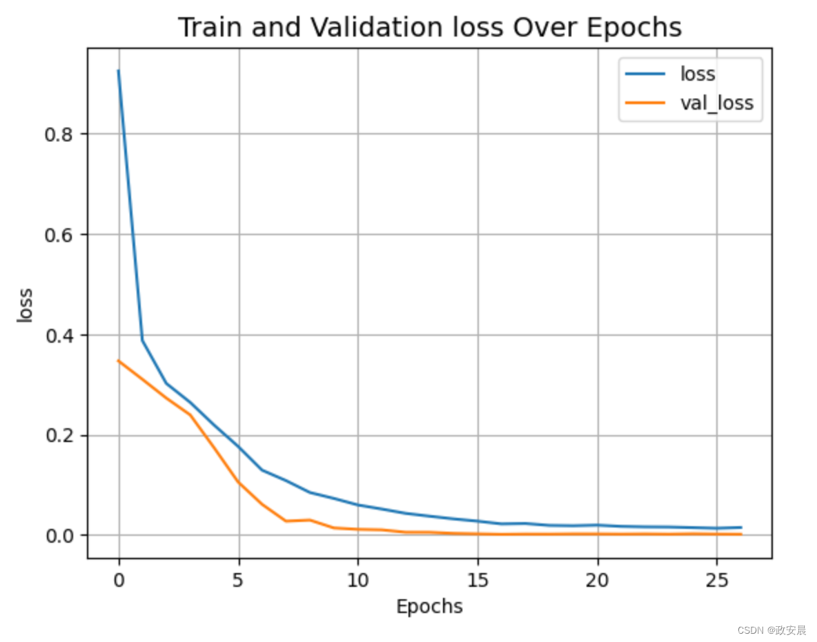
评估模型
import matplotlib.patches as patches

# Saves the model in current path
vit_object_detector.save("vit_object_detector.keras")


# To calculate IoU (intersection over union, given two bounding boxes)
def bounding_box_intersection_over_union(box_predicted, box_truth):
    # get (x, y) coordinates of intersection of bounding boxes
    top_x_intersect = max(box_predicted[0], box_truth[0])
    top_y_intersect = max(box_predicted[1], box_truth[1])
    bottom_x_intersect = min(box_predicted[2], box_truth[2])
    bottom_y_intersect = min(box_predicted[3], box_truth[3])

    # calculate area of the intersection bb (bounding box)
    intersection_area = max(0, bottom_x_intersect - top_x_intersect + 1) * max(
        0, bottom_y_intersect - top_y_intersect + 1
    )

    # calculate area of the prediction bb and ground-truth bb
    box_predicted_area = (box_predicted[2] - box_predicted[0] + 1) * (
        box_predicted[3] - box_predicted[1] + 1
    )
    box_truth_area = (box_truth[2] - box_truth[0] + 1) * (
        box_truth[3] - box_truth[1] + 1
    )

    # calculate intersection over union by taking intersection
    # area and dividing it by the sum of predicted bb and ground truth
    # bb areas subtracted by  the interesection area

    # return ioU
    return intersection_area / float(
        box_predicted_area + box_truth_area - intersection_area
    )


i, mean_iou = 0, 0

# Compare results for 10 images in the test set
for input_image in x_test[:10]:
    fig, (ax1, ax2) = plt.subplots(1, 2, figsize=(15, 15))
    im = input_image

    # Display the image
    ax1.imshow(im.astype("uint8"))
    ax2.imshow(im.astype("uint8"))

    input_image = cv2.resize(
        input_image, (image_size, image_size), interpolation=cv2.INTER_AREA
    )
    input_image = np.expand_dims(input_image, axis=0)
    preds = vit_object_detector.predict(input_image)[0]

    (h, w) = (im).shape[0:2]

    top_left_x, top_left_y = int(preds[0] * w), int(preds[1] * h)

    bottom_right_x, bottom_right_y = int(preds[2] * w), int(preds[3] * h)

    box_predicted = [top_left_x, top_left_y, bottom_right_x, bottom_right_y]
    # Create the bounding box
    rect = patches.Rectangle(
        (top_left_x, top_left_y),
        bottom_right_x - top_left_x,
        bottom_right_y - top_left_y,
        facecolor="none",
        edgecolor="red",
        linewidth=1,
    )
    # Add the bounding box to the image
    ax1.add_patch(rect)
    ax1.set_xlabel(
        "Predicted: "
        + str(top_left_x)
        + ", "
        + str(top_left_y)
        + ", "
        + str(bottom_right_x)
        + ", "
        + str(bottom_right_y)
    )

    top_left_x, top_left_y = int(y_test[i][0] * w), int(y_test[i][1] * h)

    bottom_right_x, bottom_right_y = int(y_test[i][2] * w), int(y_test[i][3] * h)

    box_truth = top_left_x, top_left_y, bottom_right_x, bottom_right_y

    mean_iou += bounding_box_intersection_over_union(box_predicted, box_truth)
    # Create the bounding box
    rect = patches.Rectangle(
        (top_left_x, top_left_y),
        bottom_right_x - top_left_x,
        bottom_right_y - top_left_y,
        facecolor="none",
        edgecolor="red",
        linewidth=1,
    )
    # Add the bounding box to the image
    ax2.add_patch(rect)
    ax2.set_xlabel(
        "Target: "
        + str(top_left_x)
        + ", "
        + str(top_left_y)
        + ", "
        + str(bottom_right_x)
        + ", "
        + str(bottom_right_y)
        + "\n"
        + "IoU"
        + str(bounding_box_intersection_over_union(box_predicted, box_truth))
    )
    i = i + 1

print("mean_iou: " + str(mean_iou / len(x_test[:10])))
plt.show()
演绎展示:
1/1 ━━━━━━━━━━━━━━━━━━━━ 1s 1s/step
 1/1 ━━━━━━━━━━━━━━━━━━━━ 0s 1ms/step
 1/1 ━━━━━━━━━━━━━━━━━━━━ 0s 1ms/step
 1/1 ━━━━━━━━━━━━━━━━━━━━ 0s 2ms/step
 1/1 ━━━━━━━━━━━━━━━━━━━━ 0s 1ms/step
 1/1 ━━━━━━━━━━━━━━━━━━━━ 0s 1ms/step
 1/1 ━━━━━━━━━━━━━━━━━━━━ 0s 1ms/step
 1/1 ━━━━━━━━━━━━━━━━━━━━ 0s 1ms/step
 1/1 ━━━━━━━━━━━━━━━━━━━━ 0s 2ms/step
 1/1 ━━━━━━━━━━━━━━━━━━━━ 0s 1ms/step
mean_iou: 0.9092338486331416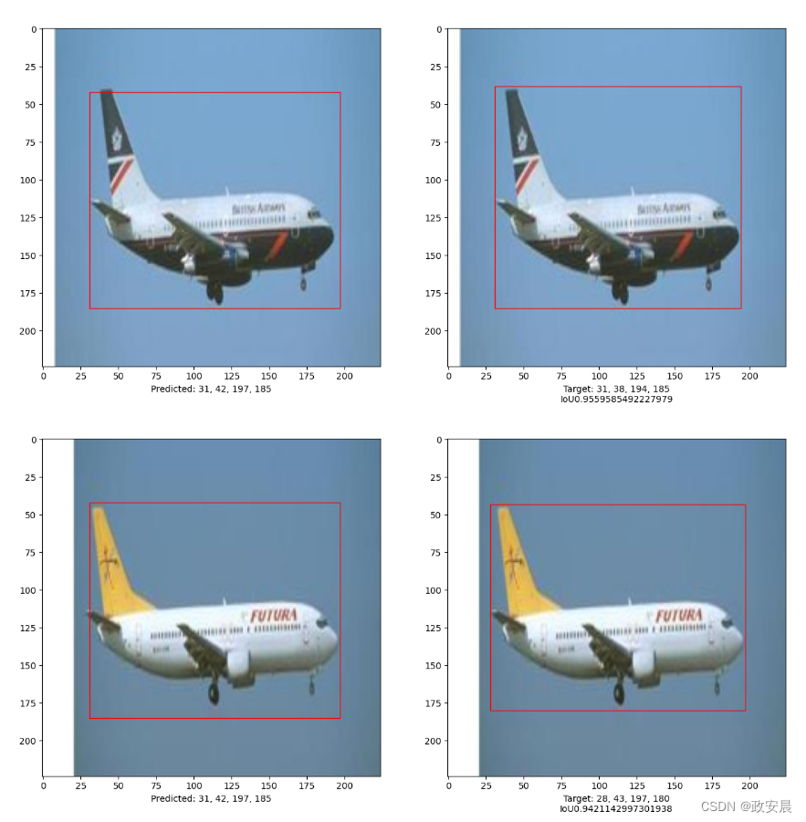
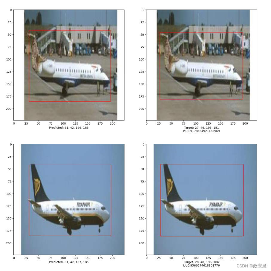


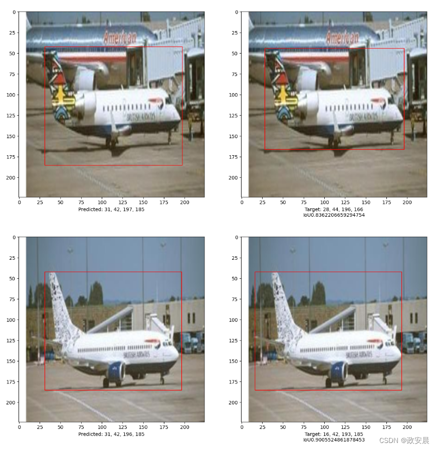
这个例子表明,可以训练一个纯变换器来预测给定图像中物体的边界框,从而将变换器的应用扩展到物体检测任务中。通过调整超参数和预训练,该模型还能得到进一步改进。


![FileNotFoundError: [Errno 2] No such file or directory: ‘llvm-config‘](https://img-blog.csdnimg.cn/direct/ba8556612b334d8c94a656517bf6e4f1.png)