PostgreSQL WITH 子句

在 PostgreSQL 中，WITH 子句提供了一种编写辅助语句的方法，以便在更大的查询中使用。

WITH 子句有助于将复杂的大型查询分解为更简单的表单，便于阅读。这些语句通常称为通用表表达式（Common Table Express， CTE），也可以当做一个为查询而存在的临时表。

WITH 子句是在多次执行子查询时特别有用，允许我们在查询中通过它的名称(可能是多次)引用它。

WITH 子句在使用前必须先定义。

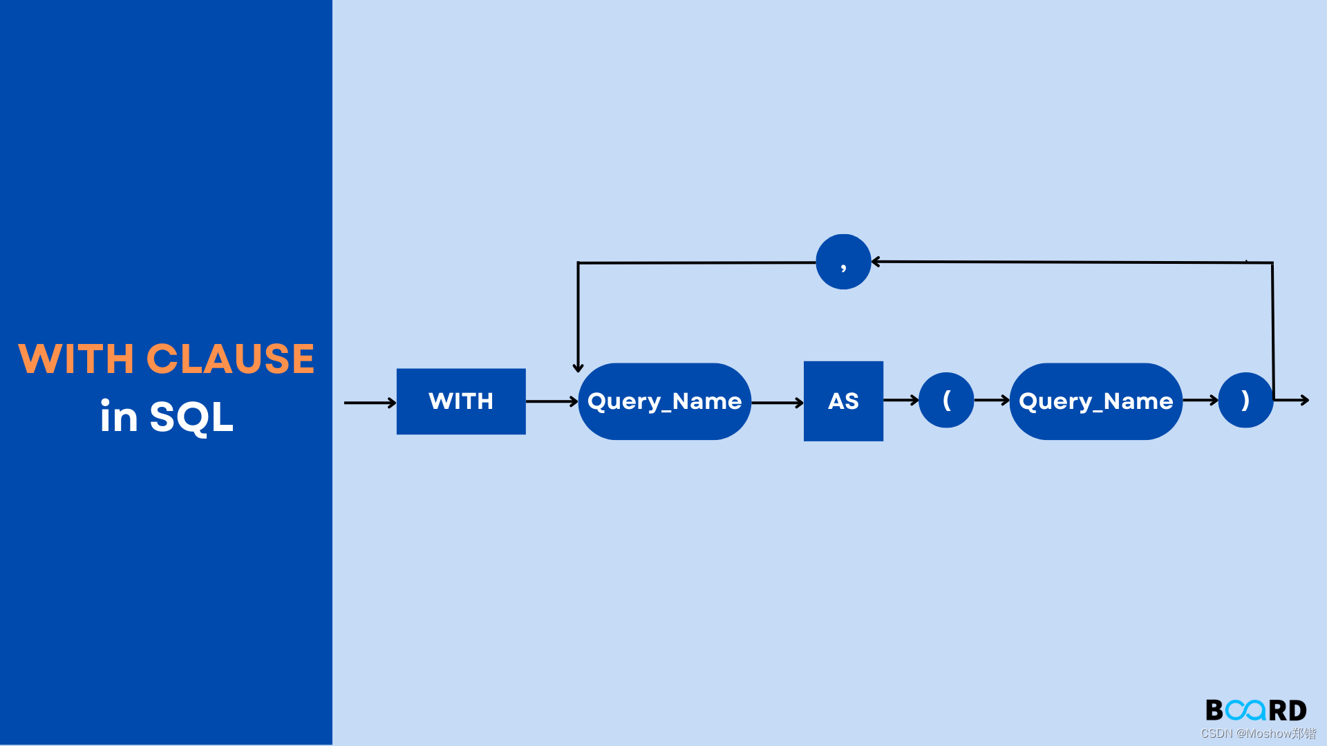
语法

WITH 查询的基础语法如下：

WITH
   name_for_summary_data AS (
      SELECT Statement)
   SELECT columns
   FROM name_for_summary_data
   WHERE conditions <=> (
      SELECT column
      FROM name_for_summary_data)
   [ORDER BY columns]

name_for_summary_data 是 WITH 子句的名称，name_for_summary_data 可以与现有的表名相同，并且具有优先级。

可以在 WITH 中使用数据 INSERT, UPDATE 或 DELETE 语句，允许您在同一个查询中执行多个不同的操作。

WITH 递归

在 WITH 子句中可以使用自身输出的数据。

公用表表达式 (CTE) 具有一个重要的优点，那就是能够引用其自身，从而创建递归 CTE。递归 CTE 是一个重复执行初始 CTE 以返回数据子集直到获取完整结果集的公用表表达式。

实例

创建 COMPANY 表（下载 COMPANY SQL 文件 ），数据内容如下：

runoobdb# select * from COMPANY;
 id | name  | age | address   | salary
----+-------+-----+-----------+--------
  1 | Paul  |  32 | California|  20000
  2 | Allen |  25 | Texas     |  15000
  3 | Teddy |  23 | Norway    |  20000
  4 | Mark  |  25 | Rich-Mond |  65000
  5 | David |  27 | Texas     |  85000
  6 | Kim   |  22 | South-Hall|  45000
  7 | James |  24 | Houston   |  10000
(7 rows)

下面将使用 WITH 子句在上表中查询数据：

With CTE AS
(Select
 ID
, NAME
, AGE
, ADDRESS
, SALARY
FROM COMPANY )
Select * From CTE;

得到结果如下：

id | name  | age | address   | salary
----+-------+-----+-----------+--------
  1 | Paul  |  32 | California|  20000
  2 | Allen |  25 | Texas     |  15000
  3 | Teddy |  23 | Norway    |  20000
  4 | Mark  |  25 | Rich-Mond |  65000
  5 | David |  27 | Texas     |  85000
  6 | Kim   |  22 | South-Hall|  45000
  7 | James |  24 | Houston   |  10000
(7 rows)

接下来让我们使用 RECURSIVE 关键字和 WITH 子句编写一个查询，查找 SALARY(工资) 字段小于 20000 的数据并计算它们的和：

WITH RECURSIVE t(n) AS (
   VALUES (0)
   UNION ALL
   SELECT SALARY FROM COMPANY WHERE SALARY < 20000
)
SELECT sum(n) FROM t;

得到结果如下：

 sum
-------
 25000
(1 row)

下面我们建立一张和 COMPANY 表相似的 COMPANY1 表，使用 DELETE 语句和 WITH 子句删除 COMPANY 表中 SALARY(工资) 字段大于等于 30000 的数据，并将删除的数据插入 COMPANY1 表，实现将 COMPANY 表数据转移到 COMPANY1 表中：

CREATE TABLE COMPANY1(
   ID INT PRIMARY KEY     NOT NULL,
   NAME           TEXT    NOT NULL,
   AGE            INT     NOT NULL,
   ADDRESS        CHAR(50),
   SALARY         REAL
);


WITH moved_rows AS (
   DELETE FROM COMPANY
   WHERE
      SALARY >= 30000
   RETURNING *
)
INSERT INTO COMPANY1 (SELECT * FROM moved_rows);

得到结果如下：

INSERT 0 3

此时，CAMPANY 表和 CAMPANY1 表的数据如下：

runoobdb=# SELECT * FROM COMPANY;
 id | name  | age |  address   | salary
----+-------+-----+------------+--------
  1 | Paul  |  32 | California |  20000
  2 | Allen |  25 | Texas      |  15000
  3 | Teddy |  23 | Norway     |  20000
  7 | James |  24 | Houston    |  10000
(4 rows)


runoobdb=# SELECT * FROM COMPANY1;
 id | name  | age | address | salary
----+-------+-----+-------------+--------
  4 | Mark  |  25 | Rich-Mond   |  65000
  5 | David |  27 | Texas       |  85000
  6 | Kim   |  22 | South-Hall  |  45000
(3 rows)

7.8. WITH Queries (Common Table Expressions) 

7.8.1. SELECT in WITH

7.8.2. Recursive Queries

7.8.3. Common Table Expression Materialization

7.8.4. Data-Modifying Statements in WITH

WITH regional_sales AS (
    SELECT region, SUM(amount) AS total_sales
    FROM orders
    GROUP BY region
), top_regions AS (
    SELECT region
    FROM regional_sales
    WHERE total_sales > (SELECT SUM(total_sales)/10 FROM regional_sales)
)
SELECT region,
       product,
       SUM(quantity) AS product_units,
       SUM(amount) AS product_sales
FROM orders
WHERE region IN (SELECT region FROM top_regions)
GROUP BY region, product;

The optional RECURSIVE modifier changes WITH from a mere syntactic convenience into a feature that accomplishes things not otherwise possible in standard SQL. Using RECURSIVE, a WITH query can refer to its own output. A very simple example is this query to sum the integers from 1 through 100:

WITH RECURSIVE t(n) AS (
    VALUES (1)
  UNION ALL
    SELECT n+1 FROM t WHERE n < 100
)
SELECT sum(n) FROM t;

The general form of a recursive WITH query is always a non-recursive term, then UNION (or UNION ALL), then a recursive term, where only the recursive term can contain a reference to the query's own output. Such a query is executed as follows:

Recursive Query Evaluation

1. Evaluate the non-recursive term. For UNION (but not UNION ALL), discard duplicate rows. Include all remaining rows in the result of the recursive query, and also place them in a temporary working table.

2. So long as the working table is not empty, repeat these steps:

   1. Evaluate the recursive term, substituting the current contents of the working table for the recursive self-reference. For UNION (but not UNION ALL), discard duplicate rows and rows that duplicate any previous result row. Include all remaining rows in the result of the recursive query, and also place them in a temporary intermediate table.

   2. Replace the contents of the working table with the contents of the intermediate table, then empty the intermediate table.

Note

While RECURSIVE allows queries to be specified recursively, internally such queries are evaluated iteratively.

In the example above, the working table has just a single row in each step, and it takes on the values from 1 through 100 in successive steps. In the 100th step, there is no output because of the WHERE clause, and so the query terminates.

Recursive queries are typically used to deal with hierarchical or tree-structured data. A useful example is this query to find all the direct and indirect sub-parts of a product, given only a table that shows immediate inclusions:

WITH RECURSIVE included_parts(sub_part, part, quantity) AS (
    SELECT sub_part, part, quantity FROM parts WHERE part = 'our_product'
  UNION ALL
    SELECT p.sub_part, p.part, p.quantity * pr.quantity
    FROM included_parts pr, parts p
    WHERE p.part = pr.sub_part
)
SELECT sub_part, SUM(quantity) as total_quantity
FROM included_parts
GROUP BY sub_part

7.8.2.1. Search Order 

When computing a tree traversal using a recursive query, you might want to order the results in either depth-first or breadth-first order. This can be done by computing an ordering column alongside the other data columns and using that to sort the results at the end. Note that this does not actually control in which order the query evaluation visits the rows; that is as always in SQL implementation-dependent. This approach merely provides a convenient way to order the results afterwards.

To create a depth-first order, we compute for each result row an array of rows that we have visited so far. For example, consider the following query that searches a table tree using a link field:

WITH RECURSIVE search_tree(id, link, data) AS (
    SELECT t.id, t.link, t.data
    FROM tree t
  UNION ALL
    SELECT t.id, t.link, t.data
    FROM tree t, search_tree st
    WHERE t.id = st.link
)
SELECT * FROM search_tree;

To add depth-first ordering information, you can write this:

WITH RECURSIVE search_tree(id, link, data, path) AS (
    SELECT t.id, t.link, t.data, ARRAY[t.id]
    FROM tree t
  UNION ALL
    SELECT t.id, t.link, t.data, path || t.id
    FROM tree t, search_tree st
    WHERE t.id = st.link
)
SELECT * FROM search_tree ORDER BY path;

In the general case where more than one field needs to be used to identify a row, use an array of rows. For example, if we needed to track fields f1 and f2:

WITH RECURSIVE search_tree(id, link, data, path) AS (
    SELECT t.id, t.link, t.data, ARRAY[ROW(t.f1, t.f2)]
    FROM tree t
  UNION ALL
    SELECT t.id, t.link, t.data, path || ROW(t.f1, t.f2)
    FROM tree t, search_tree st
    WHERE t.id = st.link
)
SELECT * FROM search_tree ORDER BY path;

Tip

Omit the ROW() syntax in the common case where only one field needs to be tracked. This allows a simple array rather than a composite-type array to be used, gaining efficiency.

To create a breadth-first order, you can add a column that tracks the depth of the search, for example:

WITH RECURSIVE search_tree(id, link, data, depth) AS (
    SELECT t.id, t.link, t.data, 0
    FROM tree t
  UNION ALL
    SELECT t.id, t.link, t.data, depth + 1
    FROM tree t, search_tree st
    WHERE t.id = st.link
)
SELECT * FROM search_tree ORDER BY depth;

To get a stable sort, add data columns as secondary sorting columns.

Tip

The recursive query evaluation algorithm produces its output in breadth-first search order. However, this is an implementation detail and it is perhaps unsound to rely on it. The order of the rows within each level is certainly undefined, so some explicit ordering might be desired in any case.

There is built-in syntax to compute a depth- or breadth-first sort column. For example:

WITH RECURSIVE search_tree(id, link, data) AS (
    SELECT t.id, t.link, t.data
    FROM tree t
  UNION ALL
    SELECT t.id, t.link, t.data
    FROM tree t, search_tree st
    WHERE t.id = st.link
) SEARCH DEPTH FIRST BY id SET ordercol
SELECT * FROM search_tree ORDER BY ordercol;

WITH RECURSIVE search_tree(id, link, data) AS (
    SELECT t.id, t.link, t.data
    FROM tree t
  UNION ALL
    SELECT t.id, t.link, t.data
    FROM tree t, search_tree st
    WHERE t.id = st.link
) SEARCH BREADTH FIRST BY id SET ordercol
SELECT * FROM search_tree ORDER BY ordercol;

This syntax is internally expanded to something similar to the above hand-written forms. The SEARCH clause specifies whether depth- or breadth first search is wanted, the list of columns to track for sorting, and a column name that will contain the result data that can be used for sorting. That column will implicitly be added to the output rows of the CTE.

7.8.2.2. Cycle Detection 

When working with recursive queries it is important to be sure that the recursive part of the query will eventually return no tuples, or else the query will loop indefinitely. Sometimes, using UNION instead of UNION ALL can accomplish this by discarding rows that duplicate previous output rows. However, often a cycle does not involve output rows that are completely duplicate: it may be necessary to check just one or a few fields to see if the same point has been reached before. The standard method for handling such situations is to compute an array of the already-visited values. For example, consider again the following query that searches a table graph using a link field:

WITH RECURSIVE search_graph(id, link, data, depth) AS (
    SELECT g.id, g.link, g.data, 0
    FROM graph g
  UNION ALL
    SELECT g.id, g.link, g.data, sg.depth + 1
    FROM graph g, search_graph sg
    WHERE g.id = sg.link
)
SELECT * FROM search_graph;

This query will loop if the link relationships contain cycles. Because we require a “depth” output, just changing UNION ALL to UNION would not eliminate the looping. Instead we need to recognize whether we have reached the same row again while following a particular path of links. We add two columns is_cycle and path to the loop-prone query:

WITH RECURSIVE search_graph(id, link, data, depth, is_cycle, path) AS (
    SELECT g.id, g.link, g.data, 0,
      false,
      ARRAY[g.id]
    FROM graph g
  UNION ALL
    SELECT g.id, g.link, g.data, sg.depth + 1,
      g.id = ANY(path),
      path || g.id
    FROM graph g, search_graph sg
    WHERE g.id = sg.link AND NOT is_cycle
)
SELECT * FROM search_graph;

Aside from preventing cycles, the array value is often useful in its own right as representing the “path” taken to reach any particular row.

In the general case where more than one field needs to be checked to recognize a cycle, use an array of rows. For example, if we needed to compare fields f1 and f2:

WITH RECURSIVE search_graph(id, link, data, depth, is_cycle, path) AS (
    SELECT g.id, g.link, g.data, 0,
      false,
      ARRAY[ROW(g.f1, g.f2)]
    FROM graph g
  UNION ALL
    SELECT g.id, g.link, g.data, sg.depth + 1,
      ROW(g.f1, g.f2) = ANY(path),
      path || ROW(g.f1, g.f2)
    FROM graph g, search_graph sg
    WHERE g.id = sg.link AND NOT is_cycle
)
SELECT * FROM search_graph;

Tip

Omit the ROW() syntax in the common case where only one field needs to be checked to recognize a cycle. This allows a simple array rather than a composite-type array to be used, gaining efficiency.

There is built-in syntax to simplify cycle detection. The above query can also be written like this:

WITH RECURSIVE search_graph(id, link, data, depth) AS (
    SELECT g.id, g.link, g.data, 1
    FROM graph g
  UNION ALL
    SELECT g.id, g.link, g.data, sg.depth + 1
    FROM graph g, search_graph sg
    WHERE g.id = sg.link
) CYCLE id SET is_cycle USING path
SELECT * FROM search_graph;

and it will be internally rewritten to the above form. The CYCLE clause specifies first the list of columns to track for cycle detection, then a column name that will show whether a cycle has been detected, and finally the name of another column that will track the path. The cycle and path columns will implicitly be added to the output rows of the CTE.

Tip

The cycle path column is computed in the same way as the depth-first ordering column show in the previous section. A query can have both a SEARCH and a CYCLE clause, but a depth-first search specification and a cycle detection specification would create redundant computations, so it's more efficient to just use the CYCLE clause and order by the path column. If breadth-first ordering is wanted, then specifying both SEARCH and CYCLE can be useful.

A helpful trick for testing queries when you are not certain if they might loop is to place a LIMIT in the parent query. For example, this query would loop forever without the LIMIT:

WITH RECURSIVE t(n) AS (
    SELECT 1
  UNION ALL
    SELECT n+1 FROM t
)
SELECT n FROM t LIMIT 100;

This works because PostgreSQL's implementation evaluates only as many rows of a WITH query as are actually fetched by the parent query. Using this trick in production is not recommended, because other systems might work differently. Also, it usually won't work if you make the outer query sort the recursive query's results or join them to some other table, because in such cases the outer query will usually try to fetch all of the WITH query's output anyway.

7.8.3. Common Table Expression Materialization 

A useful property of WITH queries is that they are normally evaluated only once per execution of the parent query, even if they are referred to more than once by the parent query or sibling WITH queries. Thus, expensive calculations that are needed in multiple places can be placed within a WITH query to avoid redundant work. Another possible application is to prevent unwanted multiple evaluations of functions with side-effects. However, the other side of this coin is that the optimizer is not able to push restrictions from the parent query down into a multiply-referenced WITH query, since that might affect all uses of the WITH query's output when it should affect only one. The multiply-referenced WITH query will be evaluated as written, without suppression of rows that the parent query might discard afterwards. (But, as mentioned above, evaluation might stop early if the reference(s) to the query demand only a limited number of rows.)

However, if a WITH query is non-recursive and side-effect-free (that is, it is a SELECT containing no volatile functions) then it can be folded into the parent query, allowing joint optimization of the two query levels. By default, this happens if the parent query references the WITH query just once, but not if it references the WITH query more than once. You can override that decision by specifying MATERIALIZED to force separate calculation of the WITH query, or by specifying NOT MATERIALIZED to force it to be merged into the parent query. The latter choice risks duplicate computation of the WITH query, but it can still give a net savings if each usage of the WITH query needs only a small part of the WITH query's full output.

A simple example of these rules is

WITH w AS (
    SELECT * FROM big_table
)
SELECT * FROM w WHERE key = 123;

This WITH query will be folded, producing the same execution plan as

SELECT * FROM big_table WHERE key = 123;

In particular, if there's an index on key, it will probably be used to fetch just the rows having key = 123. On the other hand, in

WITH w AS (
    SELECT * FROM big_table
)
SELECT * FROM w AS w1 JOIN w AS w2 ON w1.key = w2.ref
WHERE w2.key = 123;

the WITH query will be materialized, producing a temporary copy of big_table that is then joined with itself — without benefit of any index. This query will be executed much more efficiently if written as

WITH w AS NOT MATERIALIZED (
    SELECT * FROM big_table
)
SELECT * FROM w AS w1 JOIN w AS w2 ON w1.key = w2.ref
WHERE w2.key = 123;

so that the parent query's restrictions can be applied directly to scans of big_table.

An example where NOT MATERIALIZED could be undesirable is

WITH w AS (
    SELECT key, very_expensive_function(val) as f FROM some_table
)
SELECT * FROM w AS w1 JOIN w AS w2 ON w1.f = w2.f;

Here, materialization of the WITH query ensures that very_expensive_function is evaluated only once per table row, not twice.

The examples above only show WITH being used with SELECT, but it can be attached in the same way to INSERT, UPDATE, DELETE, or MERGE. In each case it effectively provides temporary table(s) that can be referred to in the main command.

7.8.4. Data-Modifying Statements in WITH 

You can use most data-modifying statements (INSERT, UPDATE, or DELETE, but not MERGE) in WITH. This allows you to perform several different operations in the same query. An example is:

WITH moved_rows AS (
    DELETE FROM products
    WHERE
        "date" >= '2010-10-01' AND
        "date" < '2010-11-01'
    RETURNING *
)
INSERT INTO products_log
SELECT * FROM moved_rows;

This query effectively moves rows from products to products_log. The DELETE in WITH deletes the specified rows from products, returning their contents by means of its RETURNING clause; and then the primary query reads that output and inserts it into products_log.

A fine point of the above example is that the WITH clause is attached to the INSERT, not the sub-SELECT within the INSERT. This is necessary because data-modifying statements are only allowed in WITH clauses that are attached to the top-level statement. However, normal WITH visibility rules apply, so it is possible to refer to the WITH statement's output from the sub-SELECT.

Data-modifying statements in WITH usually have RETURNING clauses (see Section 6.4), as shown in the example above. It is the output of the RETURNING clause, not the target table of the data-modifying statement, that forms the temporary table that can be referred to by the rest of the query. If a data-modifying statement in WITH lacks a RETURNING clause, then it forms no temporary table and cannot be referred to in the rest of the query. Such a statement will be executed nonetheless. A not-particularly-useful example is:

WITH t AS (
    DELETE FROM foo
)
DELETE FROM bar;

This example would remove all rows from tables foo and bar. The number of affected rows reported to the client would only include rows removed from bar.

Recursive self-references in data-modifying statements are not allowed. In some cases it is possible to work around this limitation by referring to the output of a recursive WITH, for example:

WITH RECURSIVE included_parts(sub_part, part) AS (
    SELECT sub_part, part FROM parts WHERE part = 'our_product'
  UNION ALL
    SELECT p.sub_part, p.part
    FROM included_parts pr, parts p
    WHERE p.part = pr.sub_part
)
DELETE FROM parts
  WHERE part IN (SELECT part FROM included_parts);

This query would remove all direct and indirect subparts of a product.

Data-modifying statements in WITH are executed exactly once, and always to completion, independently of whether the primary query reads all (or indeed any) of their output. Notice that this is different from the rule for SELECT in WITH: as stated in the previous section, execution of a SELECT is carried only as far as the primary query demands its output.

The sub-statements in WITH are executed concurrently with each other and with the main query. Therefore, when using data-modifying statements in WITH, the order in which the specified updates actually happen is unpredictable. All the statements are executed with the same snapshot (see Chapter 13), so they cannot “see” one another's effects on the target tables. This alleviates the effects of the unpredictability of the actual order of row updates, and means that RETURNING data is the only way to communicate changes between different WITH sub-statements and the main query. An example of this is that in

WITH t AS (
    UPDATE products SET price = price * 1.05
    RETURNING *
)
SELECT * FROM products;

the outer SELECT would return the original prices before the action of the UPDATE, while in

WITH t AS (
    UPDATE products SET price = price * 1.05
    RETURNING *
)
SELECT * FROM t;

the outer SELECT would return the updated data.

Trying to update the same row twice in a single statement is not supported. Only one of the modifications takes place, but it is not easy (and sometimes not possible) to reliably predict which one. This also applies to deleting a row that was already updated in the same statement: only the update is performed. Therefore you should generally avoid trying to modify a single row twice in a single statement. In particular avoid writing WITH sub-statements that could affect the same rows changed by the main statement or a sibling sub-statement. The effects of such a statement will not be predictable.

At present, any table used as the target of a data-modifying statement in WITH must not have a conditional rule, nor an ALSO rule, nor an INSTEAD rule that expands to multiple statements.

7.8. WITH查询（公共表表达式）

WITH提供了一种方式来书写在一个大型查询中使用的辅助语句。这些语句通常被称为公共表表达式或CTE，它们可以被看成是定义只在一个查询中存在的临时表。在WITH子句中的每一个辅助语句可以是一个SELECT、INSERT、UPDATE或DELETE，并且WITH子句本身也可以被附加到一个主语句，主语句也可以是SELECT、INSERT、UPDATE或DELETE。

7.8.1. WITH中的SELECT

WITH中SELECT的基本价值是将复杂的查询分解称为简单的部分。一个例子：

WITH regional_sales AS (
        SELECT region, SUM(amount) AS total_sales
        FROM orders
        GROUP BY region
     ), top_regions AS (
        SELECT region
        FROM regional_sales
        WHERE total_sales > (SELECT SUM(total_sales)/10 FROM regional_sales)
     )
SELECT region,
       product,
       SUM(quantity) AS product_units,
       SUM(amount) AS product_sales
FROM orders
WHERE region IN (SELECT region FROM top_regions)
GROUP BY region, product;

它只显示在高销售区域每种产品的销售总额。WITH子句定义了两个辅助语句regional_sales和top_regions，其中regional_sales的输出用在top_regions中而top_regions的输出用在主SELECT查询。这个例子可以不用WITH来书写，但是我们必须要用两层嵌套的子SELECT。使用这种方法要更简单些。

可选的RECURSIVE修饰符将WITH从单纯的句法便利变成了一种在标准SQL中不能完成的特性。通过使用RECURSIVE，一个WITH查询可以引用它自己的输出。一个非常简单的例子是计算从1到100的整数合的查询：

WITH RECURSIVE t(n) AS (
    VALUES (1)
  UNION ALL
    SELECT n+1 FROM t WHERE n < 100
)
SELECT sum(n) FROM t;

一个递归WITH查询的通常形式总是一个非递归项，然后是UNION（或者UNION ALL），再然后是一个递归项，其中只有递归项能够包含对于查询自身输出的引用。这样一个查询可以被这样执行：

递归查询求值

1. 计算非递归项。对UNION（但不对UNION ALL），抛弃重复行。把所有剩余的行包括在递归查询的结果中，并且也把它们放在一个临时的工作表中。

2. 只要工作表不为空，重复下列步骤：

   1. 计算递归项，用当前工作表的内容替换递归自引用。对UNION（不是UNION ALL），抛弃重复行以及那些与之前结果行重复的行。将剩下的所有行包括在递归查询的结果中，并且也把它们放在一个临时的中间表中。

   2. 用中间表的内容替换工作表的内容，然后清空中间表。

注意: 严格来说，这个处理是迭代而不是递归，但是RECURSIVE是SQL标准委员会选择的术语。

在上面的例子中，工作表在每一步只有一个行，并且它在连续的步骤中取值从1到100。在第100步，由于WHERE子句导致没有输出，因此查询终止。

递归查询通常用于处理层次或者树状结构的数据。一个有用的例子是这个用于找到一个产品的直接或间接部件的查询，只要给定一个显示了直接包含关系的表：

WITH RECURSIVE included_parts(sub_part, part, quantity) AS (
    SELECT sub_part, part, quantity FROM parts WHERE part = 'our_product'
  UNION ALL
    SELECT p.sub_part, p.part, p.quantity
    FROM included_parts pr, parts p
    WHERE p.part = pr.sub_part
  )
SELECT sub_part, SUM(quantity) as total_quantity
FROM included_parts
GROUP BY sub_part

在使用递归查询时，确保查询的递归部分最终将不返回元组非常重要，否则查询将会无限循环。在某些时候，使用UNION替代UNION ALL可以通过抛弃与之前输出行重复的行来达到这个目的。不过，经常有循环不涉及到完全重复的输出行：它可能只需要检查一个或几个域来看相同点之前是否达到过。处理这种情况的标准方法是计算一个已经访问过值的数组。例如，考虑下面这个使用link域搜索表graph的查询：

WITH RECURSIVE search_graph(id, link, data, depth) AS (
        SELECT g.id, g.link, g.data, 1
        FROM graph g
      UNION ALL
        SELECT g.id, g.link, g.data, sg.depth + 1
        FROM graph g, search_graph sg
        WHERE g.id = sg.link
)
SELECT * FROM search_graph;

如果link关系包含环，这个查询将会循环。因为我们要求一个"depth"输出，仅仅将UNION ALL 改为UNION不会消除循环。反过来在我们顺着一个特定链接路径搜索时，我们需要识别我们是否再次到达了一个相同的行。我们可以项这个有循环倾向的查询增加两个列path和cycle：

WITH RECURSIVE search_graph(id, link, data, depth, path, cycle) AS (
        SELECT g.id, g.link, g.data, 1,
          ARRAY[g.id],
          false
        FROM graph g
      UNION ALL
        SELECT g.id, g.link, g.data, sg.depth + 1,
          path || g.id,
          g.id = ANY(path)
        FROM graph g, search_graph sg
        WHERE g.id = sg.link AND NOT cycle
)
SELECT * FROM search_graph;

除了阻止环，数组值对于它们自己的工作显示到达任何特定行的"path"也有用。

在通常情况下如果需要检查多于一个域来识别一个环，请用行数组。例如，如果我们需要比较域f1和f2：

WITH RECURSIVE search_graph(id, link, data, depth, path, cycle) AS (
        SELECT g.id, g.link, g.data, 1,
          ARRAY[ROW(g.f1, g.f2)],
          false
        FROM graph g
      UNION ALL
        SELECT g.id, g.link, g.data, sg.depth + 1,
          path || ROW(g.f1, g.f2),
          ROW(g.f1, g.f2) = ANY(path)
        FROM graph g, search_graph sg
        WHERE g.id = sg.link AND NOT cycle
)
SELECT * FROM search_graph;

提示: 在通常情况下只有一个域需要被检查来识别一个环，可以省略ROW()语法。这允许使用一个简单的数组而不是一个组合类型数组，可以获得效率。

提示: 递归查询计算算法使用宽度优先搜索顺序产生它的输出。你可以通过让外部查询ORDER BY一个以这种方法构建的"path"，用来以深度优先搜索顺序显示结果。

当你不确定查询是否可能循环时，一个测试查询的有用技巧是在父查询中放一个LIMIT。例如，这个查询没有LIMIT时会永远循环：

WITH RECURSIVE t(n) AS (
    SELECT 1
  UNION ALL
    SELECT n+1 FROM t
)
SELECT n FROM t LIMIT 100;

这会起作用，因为PostgreSQL的实现只计算WITH查询中被父查询实际取到的行。不推荐在生产中使用这个技巧，因为其他系统可能以不同方式工作。同样，如果你让外层查询排序递归查询的结果或者把它们连接成某种其他表，这个技巧将不会起作用，因为在这些情况下外层查询通常将尝试取得WITH查询的所有输出。

WITH查询的一个有用的特性是在每一次父查询的执行中它们只被计算一次，即使它们被父查询或兄弟WITH查询引用了超过一次。因此，在多个地方需要的昂贵计算可以被放在一个WITH查询中来避免冗余工作。另一种可能的应用是阻止不希望的多个函数计算产生副作用。但是，从另一方面来看，优化器不能将来自父查询的约束下推到WITH查询中而不是一个普通子查询。WITH查询通常将会被按照所写的方式计算，而不抑制父查询以后可能会抛弃的行（但是，如上所述，如果对查询的引用只请求有限数目的行，计算可能会提前停止）。

以上的例子只展示了和SELECT一起使用的WITH，但是它可以被以相同的方式附加在INSERT、UPDATE或DELETE上。在每一种情况中，它实际上提供了可在主命令中引用的临时表。

7.8.2. WITH中的数据修改语句

你可以在WITH中使用数据修改语句（INSERT、UPDATE或DELETE）。这允许你在同一个查询中执行多个而不同操作。一个例子：

WITH moved_rows AS (
    DELETE FROM products
    WHERE
        "date" >= '2010-10-01' AND
        "date" < '2010-11-01'
    RETURNING *
)
INSERT INTO products_log
SELECT * FROM moved_rows;

这个查询实际上从products把行移动到products_log。WITH中的DELETE删除来自products的指定行，以它的RETURNING子句返回它们的内容，并且接着主查询读该输出并将它插入到products_log。

上述例子中好的一点是WITH子句被附加给INSERT，而没有附加给INSERT的子SELECT。这是必需的，因为数据修改语句只允许出现在附加给顶层语句的WITH子句中。不过，普通WITH可见性规则应用，这样才可能从子SELECT中引用到WITH语句的输出。

正如上述例子所示，WITH中的数据修改语句通常具有RETURNING子句。它是RETURNING子句的输出，不是数据修改语句的目标表，它形成了剩余查询可以引用的临时表。如果一个WITH中的数据修改语句缺少一个RETURNING子句，则它形不成临时表并且不能在剩余的查询中被引用。但是这样一个语句将被执行。一个非特殊使用的例子：

WITH t AS (
    DELETE FROM foo
)
DELETE FROM bar;

这个例子将从表foo和bar中移除所有行。被报告给客户端的受影响行的数目可能只包括从bar中移除的行。

数据修改语句中不允许递归自引用。在某些情况中可以采取引用一个递归WITH的输出来操作这个限制，例如：

WITH RECURSIVE included_parts(sub_part, part) AS (
    SELECT sub_part, part FROM parts WHERE part = 'our_product'
  UNION ALL
    SELECT p.sub_part, p.part
    FROM included_parts pr, parts p
    WHERE p.part = pr.sub_part
  )
DELETE FROM parts
  WHERE part IN (SELECT part FROM included_parts);

这个查询将会移除一个产品的所有直接或间接子部件。

WITH中的数据修改语句只被执行一次，并且总是能结束，而不管主查询是否读取它们所有（或者任何）的输出。注意这和WITH中SELECT的规则不同：正如前一小节所述，直到主查询要求SELECT的输出时，SELECT才会被执行。

The sub-statements in WITH中的子语句被和每一个其他子语句以及主查询并发执行。因此在使用WITH中的数据修改语句时，指定更新的顺序实际是以不可预测的方式发生的。所有的语句都使用同一个snapshot执行（参见第 13 章），因此它们不能"看见"在目标表上另一个执行的效果。这减轻了行更新的实际顺序的不可预见性的影响，并且意味着RETURNING数据是在不同WITH子语句和主查询之间传达改变的唯一方法。其例子

WITH t AS (
    UPDATE products SET price = price * 1.05
    RETURNING *
)
SELECT * FROM products;

外层SELECT可以返回在UPDATE动作之前的原始价格，而在

WITH t AS (
    UPDATE products SET price = price * 1.05
    RETURNING *
)
SELECT * FROM t;

外部SELECT将返回更新过的数据。

在一个语句中试图两次更新同一行是不被支持的。只会发生一次修改，但是该办法不能很容易地（有时是不可能）可靠地预测哪一个会被执行。这也应用于删除一个已经在同一个语句中被更新过的行：只有更新被执行。因此你通常应该避免尝试在一个语句中尝试两次修改同一个行。尤其是防止书写可能影响被主语句或兄弟子语句修改的相同行。这样一个语句的效果将是不可预测的。

当前，在WITH中一个数据修改语句中被用作目标的任何表不能有条件规则、ALSO规则或INSTEAD规则，这些规则会扩展成为多个语句。