一 VitTransformer 介绍
vit : An Image is Worth 16x16 Words: Transformers for Image Recognition at Scale
论文是基于Attention Is All You Need,由于图像数据和词数据数据格式不一样,经典的transformer不能处理图像数据,在视觉领域的应用有限。本文提出的方法可以将transformer直接应用图像分类任务,引入Patch Embedding,位置编码等方法,克服了Transformer在处理图像数据时的限制。整体流程如下。

从图中可以看出, Vision Transformer 主要有三个部分组成: 1 ) 第一部分是Linear Projection of Flattened Patches ,也就是 Emdedding 层,主要的工作就是将图像数据转换成transformer可以处理的数据格式。2)第二部分是Transformer Encoder部分,它是vit 最核心的组件(原始的NLP的transformer还有Decoder部分)。它主要是层归一化,多头注意力机制,MLP,Dropout/DropPath四个小block组成,用于学习图像数据。3) 第三部分就是MLP head ,用于分类。
二 PatchEmbedding & Positional Encoding

首先,每个图像被分割成一系列不重叠的块(16x16或者 32x32),然后做一个线性的embedding ,由于这些块如果并行的输入到transformer中,不提供位置信息,模型不知道这些块的顺序。因此要加一个 positional encoding。
在实际的实现上,图像数据是[batch_size, C , H, W] 的格式,要将其变成[batch_size , token_len , dim],其中token_len 可以理解成图像patch token的数量。以[4,3,224,224]的图像为例子,首先我们模拟分割块,对于一个图像,我们要将其分割成 (H*w)/(patch_size*patch_size)个patches,即(224x224)// (16x16) = 196个 patches 。每个patch的大小是(3,16,16),然后我们将其flatten一个768( 3x16x16)dim的 token。这样数据格式就变成[4,196,768]。
代码分割图像块 :
def split_patches(x, patch_size=16):
    batch_size, channels, height, width = x.shape
    x = x.reshape(batch_size, channels, height // patch_size, patch_size, width // patch_size, patch_size)
    x = x.permute(0, 2, 4, 1, 3, 5)
    x = x.reshape(batch_size, -1, channels * patch_size * patch_size)
    return x
当然这个过程可以通过卷积实现,官方代码其实就是用卷积来实现的。
class PatchEmbed(nn.Module) :

    def __init__(self,img_size=224,patch_size=16,in_channels=3,embed_dim=768,norm_layer=None):

        super().__init__()
        img_size = (img_size,img_size)
        patch_size = (patch_size,patch_size)
        self.img_size = img_size
        self.patch_size = patch_size
        self.grid_size = (img_size[0] // patch_size[0],img_size[1]//patch_size[1])
        self.num_patches = self.grid_size[0] * self.grid_size[1]

        # 卷积层
        self.proj = nn.Conv2d(in_channels=in_channels,out_channels=embed_dim,kernel_size=patch_size,stride=patch_size)
        # 归一化
        self.norm = norm_layer(embed_dim) if norm_layer else nn.Identity()
    def forward(self,x) :
        B,C,H,W = x.shape
        assert H == self.img_size[0] and W == self.img_size[1], \
        f"Input image size ({H}x{W} does not match input image size ({self.img_size[0]}x{self.img_size[1]}"
        x = self.proj(x).flatten(2).transpose(1,2)
        x = self.norm(x)

        return x
positional Embedding
由于输入的图像数据patch序列没有能够表达patch之间相对位置关系,因此需要加入位置编码(Positional encoding)这个特征,为了得到不同位置的对应的编码,Transformer模型使用不同频率的正余弦函数
其中 pos是表示token(flattened image patch)的位置,2i和2i+1表示位置编码向量中对应的维度,d是对应位置编码的总维度。

def add_positional_encoding(x, max_len):
    batch_size, patch_numbers, dim = x.shape
    position = torch.arange(max_len).reshape(-1, 1)
    div_term = torch.exp(torch.arange(0, dim, 2) * -(torch.log(torch.tensor(10000.0)) / dim))
    pe = torch.zeros((max_len, dim))
    pe[:, 0::2] = torch.sin(position * div_term)
    pe[:, 1::2] = torch.cos(position * div_term)
    x += pe[:patch_numbers]
    return x
三 Self-Attention
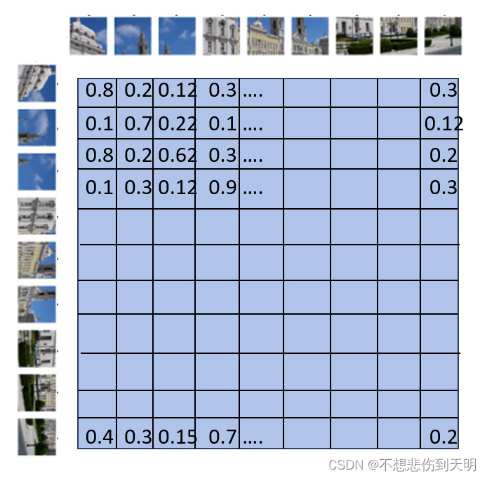
其中最核心的部分就是对于注意力部分了。在基于Transformer的机器翻译模型中,要建模源语言和目标语言任意两个单词的依赖关系,引入自注意力K(键)Q(查询)V(值)。这三个用来计算上下文单词所对应的权重得分,这些权重反映了在编码当前单词时,对于上下文不同部分所需要关注程度。
同样在vision transformer中,对于一个个image patch token 来说,也需要建模任意 token之间的相互关注关系,当处理当前token时,哪些token与它有更高的关联度。
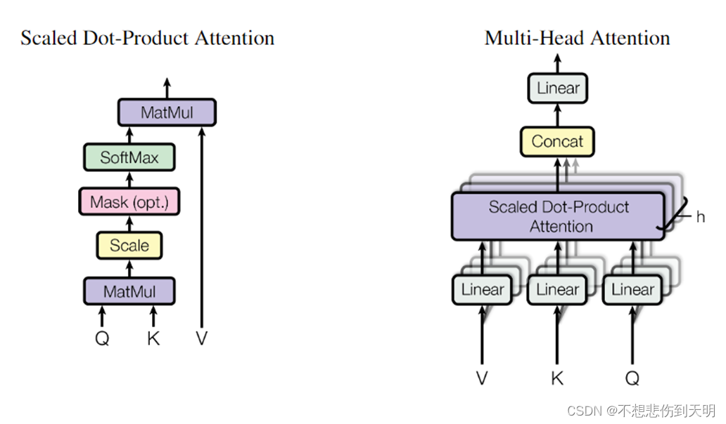
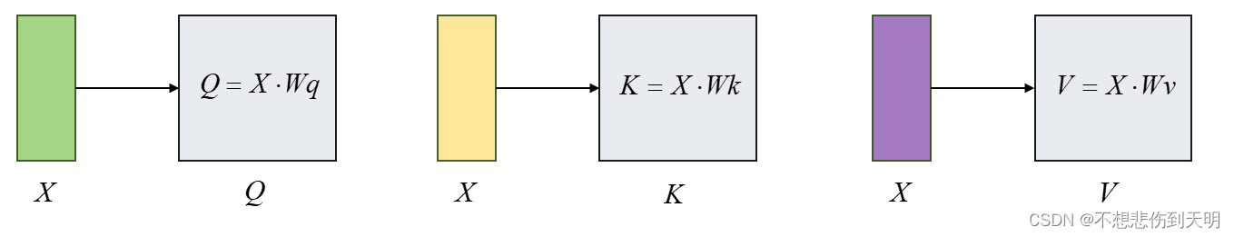
上图是论文中的Scaled Dot-Product Attention 和 Multi-head Attention,我们首先定义三个矩阵 Q,K,V,这三个矩阵是由 输入X([4,196,768])分别经过三个权重矩阵得到的。其中 Q 矩阵和K 矩阵,V矩阵是“同源”的,因为它们都是来自于同一个输入序列(图像patch token)的某种表示(线性变换的嵌入表示)。
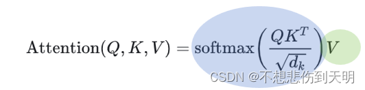
根据Attenton分数的计算公式,Q(shape=[4,196,768])左乘一个K(shape=[4,196,768])矩阵的转置,得到一个相似度矩阵(shape=[4,196,196]),为了防止过大的相似度数值在后续Softmax计算过程中导致的梯度爆炸以及收敛效率差的问题,因此使用一个缩放因子缩放来稳定优化。放缩后的得分经过Softmax函数归一化为概率后,与其他位置的值向量相乘来聚合希望关注的上下文信息,并最小化不相关信息的干扰。
def self_attention(x, w_q, w_k, w_v):
    query = torch.matmul(x, w_q)
    key = torch.matmul(x, w_k)
    value = torch.matmul(x, w_v)
    scores = torch.matmul(query, key.transpose(-2, -1)) / torch.sqrt(torch.tensor(query.shape[-1], dtype=torch.float32))
    attention_scores = softmax(scores)
    output = torch.matmul(attention_scores, value)
    return attention_scores, output
过程如下

四 Multi-head self-attention (MSA)
为了进一步提升自注意力机制的全局信息聚合能力,提出了Multi-head attention机制,具体来说,上下文的每个token 向量的表示的经过多组的线性
映射到不同的表示子空间。计算出不同子空间得到的attention score得到
,再用一个线性变换
用于综合不同子空间中的上下文表示形成最后的输出。

import torch
import torch.nn.functional as F

class MultiHeadAttention(torch.nn.Module):
    def __init__(self, input_dim, num_heads, head_dim):
        super(MultiHeadAttention, self).__init__()
        self.num_heads = num_heads
        self.head_dim = head_dim

        assert input_dim % self.num_heads == 0
        self.projection_dim = input_dim // self.num_heads

       # 定义 权重矩阵
        self.weight_q = torch.nn.Parameter(torch.randn(num_heads, input_dim, self.projection_dim))
        self.weight_k = torch.nn.Parameter(torch.randn(num_heads, input_dim, self.projection_dim))
        self.weight_v = torch.nn.Parameter(torch.randn(num_heads, input_dim, self.projection_dim))


        self.weight_combine = torch.nn.Parameter(torch.randn(num_heads * self.projection_dim, input_dim))

    def forward(self, x):
        batch_size, seq_length, _ = x.size()


        queries = torch.matmul(x, self.weight_q)
        keys = torch.matmul(x, self.weight_k)
        values = torch.matmul(x, self.weight_v)


        queries = queries.view(batch_size, seq_length, self.num_heads, self.projection_dim)
        keys = keys.view(batch_size, seq_length, self.num_heads, self.projection_dim)
        values = values.view(batch_size, seq_length, self.num_heads, self.projection_dim)


        queries = queries.transpose(1, 2)
        keys = keys.transpose(1, 2)
        values = values.transpose(1, 2)

        # 计算得分
        scores = torch.matmul(queries, keys.transpose(-2, -1)) / (self.projection_dim ** 0.5)
        attention_weights = F.softmax(scores, dim=-1)
        attention_output = torch.matmul(attention_weights, values)

        attention_output = attention_output.transpose(1, 2).contiguous().view(batch_size, seq_length, -1)
        output = torch.matmul(attention_output, self.weight_combine)

        return output

input_dim = 64
num_heads = 8
head_dim = input_dim // num_heads
seq_length = 10
batch_size = 4


multihead_attention = MultiHeadAttention(input_dim, num_heads, head_dim)
x = torch.rand(batch_size, seq_length, input_dim)
output = multihead_attention(x)

print("输入形状:", x.shape)
print("输出形状:", output.shape)
五 代码实现
import torch
import matplotlib.pyplot as plt
from PIL import Image
from torchvision.transforms import transforms
import numpy as np

def softmax(x):
    return torch.nn.functional.softmax(x, dim=-1)

def split_patches(x, patch_size=16):
    batch_size, channels, height, width = x.shape
    x = x.reshape(batch_size, channels, height // patch_size, patch_size, width // patch_size, patch_size)
    x = x.permute(0, 2, 4, 1, 3, 5)
    x = x.reshape(batch_size, -1, channels * patch_size * patch_size)
    return x

def add_positional_encoding(x, max_len):
    batch_size, patch_numbers, dim = x.shape
    position = torch.arange(max_len).reshape(-1, 1)
    div_term = torch.exp(torch.arange(0, dim, 2) * -(torch.log(torch.tensor(10000.0)) / dim))
    pe = torch.zeros((max_len, dim))
    pe[:, 0::2] = torch.sin(position * div_term)
    pe[:, 1::2] = torch.cos(position * div_term)
    x += pe[:patch_numbers]
    return x

def plot_heatmap(scores,index,name ):
    plt.figure(figsize=(8, 6))
    plt.imshow(scores, cmap='hot', interpolation='nearest')
    plt.xlabel('Keys')
    plt.ylabel('Queries')
    plt.title(f'Attention Scores Heatmap {name}')
    plt.colorbar()
    plt.savefig(f"./attention_heatmap{index}.png")
    # plt.show()
def self_attention(x, w_q, w_k, w_v):
    query = torch.matmul(x, w_q)
    key = torch.matmul(x, w_k)
    value = torch.matmul(x, w_v)
    scores = torch.matmul(query, key.transpose(-2, -1)) / torch.sqrt(torch.tensor(query.shape[-1], dtype=torch.float32))
    attention_scores = softmax(scores)
    output = torch.matmul(attention_scores, value)
    return attention_scores, output

def plot_heatmap_on_image(image, attention_scores, patch_size=16,index=0):
    # 对每个patch的注意力分数求平均
    attention_scores_mean = attention_scores.mean(dim=1)
    # 将注意力分数转换为与原始图像大小相匹配的热力图
    attention_map = attention_scores_mean.view(1, 1, int(224 / patch_size), int(224 / patch_size))
    attention_map = torch.nn.functional.interpolate(attention_map, size=(224, 224), mode='bilinear', align_corners=False)
    attention_map = attention_map.squeeze().cpu().detach().numpy()


    plt.figure(figsize=(6, 6))
    plt.imshow(image)
    plt.imshow(attention_map, cmap='jet', alpha=0.5)
    plt.axis('off')
    plt.savefig(f'attention_map{index}.png')
    # plt.show()

if __name__ == '__main__':
    batch_size = 4
    channels = 3
    height = 224
    width = 224
    input_dim = 768
    output_dim = 64

    transform = transforms.Compose([
        transforms.Resize((224, 224)),
        transforms.ToTensor()
    ])


    image_paths = ["./images/11.jpg",
                   "./images/15.jpg",
                   "./images/16.jpg",
                   "./images/17.jpg"]

    images = torch.zeros((4, 3, 224, 224), dtype=torch.float32)
    for i, path in enumerate(image_paths):
        img = Image.open(path).convert('RGB')
        img_tensor = transform(img)
        images[i] = img_tensor


    patch_embeddings = split_patches(images, patch_size=16)
    patch_embeddings_pe = add_positional_encoding(patch_embeddings, max_len=196)

    w_q = torch.normal(0, 0.01, size=(input_dim, output_dim))
    w_k = torch.normal(0, 0.01, size=(input_dim, output_dim))
    w_v = torch.normal(0, 0.01, size=(input_dim, output_dim))

    attention_scores, output = self_attention(patch_embeddings_pe, w_q, w_k, w_v)

    # plot_heatmap(attention_scores[0])
    # for index in range(4) :
    #
    #     name = image_paths[index].split('/')[-1].split('.')[0]
    #     plot_heatmap(attention_scores[index],index,name)  # 选择第一张图像的注意力分数进行绘制


    # 将热力图叠加到原始图像上
    for index in range(4) :
        image_path = image_paths[index]
        img = Image.open(image_path).convert('RGB')
        img_tensor = transform(img)

        img_np = np.array(img)

        plot_heatmap_on_image(img_np, attention_scores[index],16,index=index)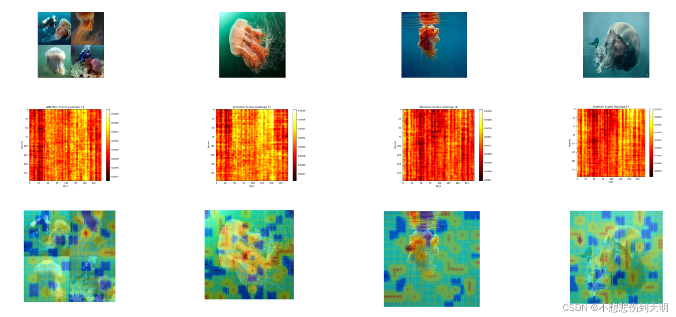
参考
-
LLM(廿四):Transformer 的结构改进与替代方案 - 知乎
-
【深度学习系列】五、Self Attention_self attention 加入位置信息-CSDN博客
-
NLP(五):Transformer及其attention机制 - 知乎
-
有关vision transformer的一个综述 - 知乎
-
为什么 Vision transformer 训练和推理很慢? - 知乎
-
大规模语言模型:从理论到实践 -- 张奇、桂韬、郑锐、黄萱菁


![每日一题 --- 删除链表的倒数第 N 个结点[力扣][Go]](https://img-blog.csdnimg.cn/img_convert/f8f8838f486669d6071ffdfec2e76c4e.jpeg)