前言
SQL查询当中,In和Exists子查询到底有无区别?记得很多年以前,确实是有相关的使用戒条的,或者说存在一些使用的惯用法。试图完全抹开两者的区别,就有点过了。
两者的主要区别:
从目的上讲,IN和EXISTS都是SQL中用于子查询的操作符。
IN操作符是用来检查一个值是否在一组值中。例如SELECT * FROM Customers WHERE Country IN ('Germany', 'France', 'UK')
EXISTS操作符是用来检查一个子查询是否至少返回一个记录。例如:SELECT * FROM Products WHERE EXISTS (SELECT * FROM OrderDetails WHERE Products.ProductID = OrderDetails.ProductID)
基本的区别还有:
1. 语义上的区别:IN关键字用来查询在某个列表中的数据,EXISTS关键字用来查询是否存在子查询返回的数据。
2. 性能上的区别:在数据量大时,或者进行全表扫描的时候,EXISTS的性能通常优于IN。因为EXISTS只要找到一个满足条件的就不再继续查询,而IN需要查询所有可能的结果。
3. 返回结果的差异:IN只能操作单个字段,EXISTS可以操作多个字段。
使用原则,主要有以下几点:
1. 当子查询返回的结果集非常大的时候,建议使用EXISTS,因为对于EXISTS来说,只要存在就会停止查询,效率更高。
2. 当子查询返回的结果集非常小,主查询的结果集非常大或是需要在结果集内进行查询时优先考虑IN。
3. 当需要比较的是多个字段而非单个字段时,应使用EXISTS。
4. 避免在子查询中使用排序操作,因为无论是IN还是EXISTS都会忽略排序,数据库还为此额外消耗资源。
上边是从ChatGPT里头摘出来的。但是对于PG而言,中间的一些结论未必正确。首先,PG是支持多列进行IN筛选的。下边我们通过简单的例子进行验证。
实例
1、关于多列在IN中是否支持?
create table a(id int primary key, col2 int);
insert into a values(1, 1);
select * from a where id in (1, 2);
select * from a where (id, col2) in (select 1, 1)  -- 4
-- select * from a where (id, col2) in (1, 2) -- 5 // 这个语句是不对,不是想象中的那样
如果你拿上边的SQL语句去各DB中去试,大多数DBMS是不支持第4个语句的语法的。比如你在SQLServer2022中,会报如下的错误:
Msg 4145 Level 15 State 1 Line 4
An expression of non-boolean type specified in a context where a condition is expected, near ','.
Sybase ASE那就更不支持了。
MySQL和PostgreSQL是支持的。甚至SQLite也是不支持的。报的错:**Query Error:** Error: SQLITE_ERROR: near ";": syntax error
Oracle号称宇宙最强,看起来是下边这个样子,同样不支持:
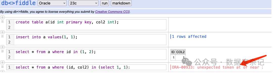
它提示的错,也是比较的含糊。
我们来看看相对强大的PostgreSQL对于多列的支持:
postgres=# select * from a where (id, col2) in (select 1,1);
 id | col2
----+------
  1 |    1
(1 row)
postgres=# select * from a where (id, col2) in (1, 2);
ERROR:  operator does not exist: record = integer
LINE 1: select * from a where (id, col2) in (1, 2);
                                         ^
HINT:  No operator matches the given name and argument types. You might need to add explicit type casts.
Time: 0.397 ms
既然PG支持,放心大胆的使用就行了。
2、NULL值的处理
这个应该是共性问题。假设表 c (id int, col2 int) , d(id int, col2 int), 其结构如下:
create table c(id int primary key, col2 int);
create table d(id int primary key, col2 int);
insert into c values(1, 1), (2, null);
insert into d values(1, 1), (3, null);
我们看看IN和exists两种操作的区别:
postgres=# select * from c where col2 in (select col2 from d);
 id | col2
----+------
  1 |    1
(1 row)

Time: 0.702 ms
postgres=# select * from c where col2 not in (select col2 from d);
 id | col2
----+------
(0 rows)
针对NULL值, IN和NOT IN都是false
postgres=# select * from c where exists (select col2 from d where d.col2 = c.col2);
 id | col2
----+------
  1 |    1
(1 row)

Time: 0.706 ms
postgres=# select * from c where not exists (select col2 from d where d.col2 = c.col2);
 id | col2
----+------
  2 |
(1 row)
Exists 子句好理解,= 操作不适用于NULL, 所以NULL值关联的行被排除。但是not exists就不一样了,它会把NULL值相关行给算在内。实际上就是一个存在性的判断。把前边符合存在条件的那些行给排除了就是最后结果。
3、主表子表的应用原则
3.1、子查询返回值比较少的情形
-- 往 a 表插入500010条记录
\timing
postgres=# insert into a select n, 99000 * random() from generate_series(1, 500000) as n;
INSERT 0 500000
Time: 1023.998 ms (00:01.024)
postgres=# insert into a select n, 99001 + 10 * random() from generate_series(500001, 500010) as n;
INSERT 0 10
Time: 1.796 ms

-- 往 b 表 插入 50000条记录
postgres=# insert into b select n, 100000 + 99000 * random() from generate_series(1, 49990) as n;
INSERT 0 49990
Time: 196.378 ms
postgres=# insert into b select n, 99001 + (n-49990) from generate_series(49991, 50000) as n;
INSERT 0 10
Time: 1.402 ms

-- 创建合达的索引
postgres=# create index idx_col2_a on a(col2);
CREATE INDEX
Time: 412.309 ms
postgres=# create index idx_col2_b on b(col2);
ERROR:  relation "idx_col2_b" already exists
Time: 0.589 ms
这里a为500010条记录,b表仅为5000条记录。它们在col2上进行存在性选择。我们看看效果:
-- 子查询建立在b表上:
ostgres=# select * from a where col2 in (select col2 from b);
   id   | col2
--------+-------
 500001 | 99006
 500002 | 99006
 500003 | 99007
 500004 | 99003
 500005 | 99004
 500006 | 99004
 500008 | 99007
 500009 | 99010
 500010 | 99009
(9 rows)

Time: 119.565 ms

postgres=# select * from a where exists (select col2 from b where b.col2 = a.col2);
   id   | col2
--------+-------
 500001 | 99006
 500002 | 99006
 500003 | 99007
 500004 | 99003
 500005 | 99004
 500006 | 99004
 500008 | 99007
 500009 | 99010
 500010 | 99009
(9 rows)

Time: 91.205 ms

-- 子表在a上:
postgres=# select * from b where col2 in (select col2 from a);
  id   | col2
-------+-------
 49992 | 99003
 49993 | 99004
 49995 | 99006
 49996 | 99007
 49998 | 99009
 49999 | 99010
(6 rows)

Time: 41.531 ms
postgres=# select * from b where exists (select col2 from a where a.col2 = b.col2);
  id   | col2
-------+-------
 49992 | 99003
 49993 | 99004
 49995 | 99006
 49996 | 99007
 49998 | 99009
 49999 | 99010
(6 rows)

Time: 73.370 ms
实际上多查几次,你会发现,两者时间上差不多。
而比较查询计划,你也看到用到的几乎是同一个查询计划。这就是在pg中的表现。
看看Not IN, Not Exists:
-- 主表为a
postgres=# select count(*) from a where col2 not in (select col2 from b where a.col2 = b.col2);
 count
--------
 500001
(1 row)

Time: 484.076 ms
postgres=# select count(*) from a where not exists (select col2 from b where a.col2=b.col2);
 count
--------
 500001
(1 row)

Time: 108.899 ms

-- 主表为b
postgres=# select count(*) from b where col2 not in (select col2 from a where a.col2 = b.col2);
 count
-------
 49994
(1 row)

Time: 50.395 ms
postgres=# select count(*) from b where not exists (select col2 from a where a.col2 = b.col2);
 count
-------
 49994
(1 row)

Time: 182.841 ms
从上边的结果来看,基本上区别也不是很明显。这是在子查询的结果集比较小的情况下:只有9个值。如果子查询的结果非常大,有可能得到的结论就不太一样。
不失一般性,采用上边列出的使用原则没有什么坏处。
3.2、子查询返回结果比较多的情形
接上边,把a, b清空,换上公共值比较多的情形,看看是啥效果?
truncate a, b;

postgres=# insert into a select n, 10000* random() from generate_series(1, 500000) as n;
INSERT 0 500000
postgres=# insert into b select n, 10000* random() from generate_series(1, 50000) as n;
INSERT 0 50000

\timing on

-- a 用作主查询
-- 使用 IN
postgres=# explain (analyze, costs) select count(*) from a where a.col2 in (select col2 from b);
                                                                QUERY PLAN
------------------------------------------------------------------------------------------------------------------------------------------
 Finalize Aggregate  (cost=11894.74..11894.75 rows=1 width=8) (actual time=197.636..197.688 rows=1 loops=1)
   ->  Gather  (cost=11894.63..11894.74 rows=1 width=8) (actual time=195.523..197.678 rows=2 loops=1)
         Workers Planned: 1
         Workers Launched: 1
         ->  Partial Aggregate  (cost=10894.63..10894.64 rows=1 width=8) (actual time=183.432..183.436 rows=1 loops=2)
               ->  Hash Join  (cost=1065.25..10178.45 rows=286469 width=0) (actual time=22.662..144.762 rows=248460 loops=2)
                     Hash Cond: (a.col2 = b.col2)
                     ->  Parallel Seq Scan on a  (cost=0.00..5154.18 rows=294118 width=4) (actual time=0.008..16.545 rows=250000 loops=2)
                     ->  Hash  (cost=944.00..944.00 rows=9700 width=4) (actual time=22.585..22.587 rows=9939 loops=2)
                           Buckets: 16384  Batches: 1  Memory Usage: 478kB
                           ->  HashAggregate  (cost=847.00..944.00 rows=9700 width=4) (actual time=20.098..21.235 rows=9939 loops=2)
                                 Group Key: b.col2
                                 Batches: 1  Memory Usage: 913kB
                                 Worker 0:  Batches: 1  Memory Usage: 913kB
                                 ->  Seq Scan on b  (cost=0.00..722.00 rows=50000 width=4) (actual time=0.013..11.360 rows=50000 loops=2)
 Planning Time: 0.268 ms
 Execution Time: 197.841 ms
(17 rows)

Time: 198.537 ms

-- 使用EXISTS
postgres=# explain (analyze, costs) select count(*) from a where exists (select * from b where a.col2 = b.col2);
                                                                QUERY PLAN
------------------------------------------------------------------------------------------------------------------------------------------
 Finalize Aggregate  (cost=11894.74..11894.75 rows=1 width=8) (actual time=192.080..192.130 rows=1 loops=1)
   ->  Gather  (cost=11894.63..11894.74 rows=1 width=8) (actual time=189.941..192.118 rows=2 loops=1)
         Workers Planned: 1
         Workers Launched: 1
         ->  Partial Aggregate  (cost=10894.63..10894.64 rows=1 width=8) (actual time=177.449..177.452 rows=1 loops=2)
               ->  Hash Join  (cost=1065.25..10178.45 rows=286469 width=0) (actual time=21.696..148.908 rows=248460 loops=2)
                     Hash Cond: (a.col2 = b.col2)
                     ->  Parallel Seq Scan on a  (cost=0.00..5154.18 rows=294118 width=4) (actual time=0.010..38.817 rows=250000 loops=2)
                     ->  Hash  (cost=944.00..944.00 rows=9700 width=4) (actual time=21.598..21.600 rows=9939 loops=2)
                           Buckets: 16384  Batches: 1  Memory Usage: 478kB
                           ->  HashAggregate  (cost=847.00..944.00 rows=9700 width=4) (actual time=19.178..20.280 rows=9939 loops=2)
                                 Group Key: b.col2
                                 Batches: 1  Memory Usage: 913kB
                                 Worker 0:  Batches: 1  Memory Usage: 913kB
                                 ->  Seq Scan on b  (cost=0.00..722.00 rows=50000 width=4) (actual time=0.015..11.202 rows=50000 loops=2)
 Planning Time: 0.330 ms
 Execution Time: 192.297 ms
(17 rows)

Time: 193.106 ms

两者差不多。

-- 再看NOT IN
postgres=# explain (analyze, costs) select count(*) from a where a.col2 not in (select col2 from b);
                                                              QUERY PLAN
--------------------------------------------------------------------------------------------------------------------------------------
 Finalize Aggregate  (cost=8104.23..8104.24 rows=1 width=8) (actual time=154.519..154.575 rows=1 loops=1)
   ->  Gather  (cost=8104.12..8104.23 rows=1 width=8) (actual time=152.256..154.562 rows=2 loops=1)
         Workers Planned: 1
         Workers Launched: 1
         ->  Partial Aggregate  (cost=7104.12..7104.13 rows=1 width=8) (actual time=139.397..139.398 rows=1 loops=2)
               ->  Parallel Seq Scan on a  (cost=847.00..6736.47 rows=147059 width=0) (actual time=21.763..139.242 rows=1540 loops=2)
                     Filter: (NOT (hashed SubPlan 1))
                     Rows Removed by Filter: 248460
                     SubPlan 1
                       ->  Seq Scan on b  (cost=0.00..722.00 rows=50000 width=4) (actual time=0.023..11.494 rows=50000 loops=2)
 Planning Time: 0.187 ms
 Execution Time: 154.649 ms
(12 rows)

Time: 155.277 ms

postgres=# explain (analyze, costs) select count(*) from a where not exists  (select * from b where b.col2 = a.col2);
                                                                             QUERY PLAN

-----------------------------------------------------------------------------------------------------------------------------------------------------------
---------
 Finalize Aggregate  (cost=9686.56..9686.57 rows=1 width=8) (actual time=143.476..144.009 rows=1 loops=1)
   ->  Gather  (cost=9686.44..9686.55 rows=1 width=8) (actual time=143.468..144.001 rows=2 loops=1)
         Workers Planned: 1
         Workers Launched: 1
         ->  Partial Aggregate  (cost=8686.44..8686.45 rows=1 width=8) (actual time=130.231..130.235 rows=1 loops=2)
               ->  Parallel Hash Anti Join  (cost=1268.06..8667.32 rows=7649 width=0) (actual time=6.437..130.089 rows=1540 loops=2)
                     Hash Cond: (a.col2 = b.col2)
                     ->  Parallel Seq Scan on a  (cost=0.00..5154.18 rows=294118 width=4) (actual time=0.008..34.314 rows=250000 loops=2)
                     ->  Parallel Hash  (cost=900.41..900.41 rows=29412 width=4) (actual time=5.975..5.976 rows=25000 loops=2)
                           Buckets: 65536  Batches: 1  Memory Usage: 2496kB
                           ->  Parallel Index Only Scan using idx_col2_b on b  (cost=0.29..900.41 rows=29412 width=4) (actual time=0.022..4.175 rows=50000
loops=1)
                                 Heap Fetches: 0
 Planning Time: 0.351 ms
 Execution Time: 144.057 ms
(14 rows)

Time: 144.851 ms
a 作主查询时,没看到有特别大的区别。
再看看如果b用作主表时的情况:
postgres=# select count(*) from b where b.col2 in (select col2 from a);
 count
-------
 50000
(1 row)

Time: 122.761 ms
postgres=# select count(*) from b where exists (select * from a where a.col2 = b.col2);
 count
-------
 50000
(1 row)

Time: 102.271 ms

postgres=# select count(*) from b where b.col2 not in (select col2 from a);
 count
-------
     0
(1 row)

Time: 46994.345 ms (00:46.994)

ostgres=# select count(*) from b where not exists (select * from a where a.col2=b.col2);
 count
-------
     0
(1 row)

Time: 169.132 ms

-- 取两者的查询计划看下:
postgres=# explain (analyze, costs) select count(*) from b where b.col2 not in (select col2 from a);
                                                                            QUERY PLAN

-----------------------------------------------------------------------------------------------------------------------------------------------------------
-------
 Finalize Aggregate  (cost=189957893.17..189957893.18 rows=1 width=8) (actual time=75657.828..75657.991 rows=1 loops=1)
   ->  Gather  (cost=189957893.05..189957893.16 rows=1 width=8) (actual time=75127.117..75657.979 rows=2 loops=1)
         Workers Planned: 1
         Workers Launched: 1
         ->  Partial Aggregate  (cost=189956893.05..189956893.06 rows=1 width=8) (actual time=75379.382..75379.384 rows=1 loops=2)
               ->  Parallel Index Only Scan using idx_col2_b on b  (cost=0.29..189956856.29 rows=14706 width=0) (actual time=75379.372..75379.373 rows=0 lo
ops=2)
                     Filter: (NOT (SubPlan 1))
                     Rows Removed by Filter: 25000
                     Heap Fetches: 0
                     SubPlan 1
                       ->  Materialize  (cost=0.00..11667.00 rows=500000 width=4) (actual time=0.002..1.906 rows=10013 loops=50000)
                             ->  Seq Scan on a  (cost=0.00..7213.00 rows=500000 width=4) (actual time=0.004..1.645 rows=9965 loops=15953)
 Planning Time: 0.244 ms
 Execution Time: 75658.697 ms
(14 rows)

Time: 75659.529 ms (01:15.660)

postgres=# explain (analyze, costs) select count(*) from b where not exists (select * from a where a.col2=b.col2);
                                                                       QUERY PLAN
--------------------------------------------------------------------------------------------------------------------------------------------------------
 Aggregate  (cost=13479.75..13479.76 rows=1 width=8) (actual time=188.005..191.547 rows=1 loops=1)
   ->  Gather  (cost=10979.94..13479.75 rows=1 width=0) (actual time=187.996..191.537 rows=0 loops=1)
         Workers Planned: 1
         Workers Launched: 1
         ->  Parallel Hash Anti Join  (cost=9979.94..12479.65 rows=1 width=0) (actual time=174.642..174.646 rows=0 loops=2)
               Hash Cond: (b.col2 = a.col2)
               ->  Parallel Index Only Scan using idx_col2_b on b  (cost=0.29..900.41 rows=29412 width=4) (actual time=0.035..2.130 rows=25000 loops=2)
                     Heap Fetches: 0
               ->  Parallel Hash  (cost=5154.18..5154.18 rows=294118 width=4) (actual time=125.958..125.959 rows=250000 loops=2)
                     Buckets: 131072  Batches: 8  Memory Usage: 3552kB
                     ->  Parallel Seq Scan on a  (cost=0.00..5154.18 rows=294118 width=4) (actual time=0.016..67.203 rows=250000 loops=2)
 Planning Time: 0.488 ms
 Execution Time: 191.611 ms
(13 rows)

Time: 192.691 ms
我们会发现,在使用not in时,将大表大结果集放到子查询里头,它花了差不多46秒的时间。这显然是不被推荐的。而not exists则显得相对稳定。
基于此,我仍然认为上边推荐的使用原则还是值得遵守的。
4、奇葩的现象
有时候,会出现在“手误”的情况下:
create table d (id int primary key, col2 int);
create table e (id int primary key, col3 int);
insert into d values(1, 1), (3, null);
insert into e values(1, 1);

postgres=# select * from d where col2 in (select col2 from e);
 id | col2
----+------
  1 |    1
(1 row)

Time: 0.512 ms
postgres=# select * from d where col2 not in (select col2 from e);
 id | col2
----+------
(0 rows)

postgres=# select * from d where exists (select col2 from e);
 id | col2
----+------
  1 |    1
  3 |
(2 rows)

ostgres=# select * from d where exists (select col2 from e where e.col2 = d.col2);
ERROR:  column e.col2 does not exist
LINE 1: ...t * from d where exists (select col2 from e where e.col2 = d...
                                                             ^
HINT:  Perhaps you meant to reference the column "e.col3" or the column "d.col2".
Time: 0.402 ms
你会发现,在加了where条件之后,它才会去校验是否真有那个列。
总结:
子查询涉及到NULL值时,需要小心注意NOT IN, NOT exists。实际使用的时候,估然需要结合查询计划以及子查询的结果集大小来进行综合判断。个人认为,要尽量慎用NOT IN。PG是支持IN的多字段子查询的。这个用起来也是很方便的。跨数据库移植时,那还是考虑使用exists的能用形式为宜。