学习笔记自,慕课网 《Python3 入门人工智能》
https://coding.imooc.com/lesson/418.html#mid=32716
分类问题
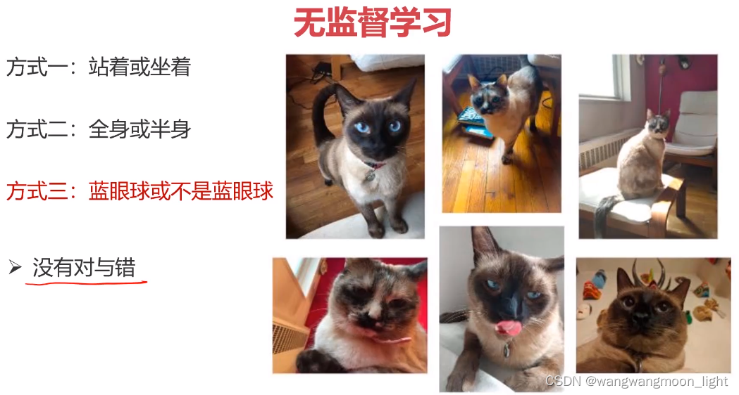
1. 无监督学习
机器学习的一种方法,没有给定事先标记过的训练示例,自动对输入的数据进行分类或分群
优点:
1)算法不受监督信息的约束,可能考虑到新的信息
2)不需要标签数据,极大程度扩大数据样本
主要应用:聚类分析、关联规则、维度缩减

聚类分析,又称为群分析,根据对象某些属性的相似度,将其自动化分为不同的类别

2. KMeans、KNN、Mean-shift
2.1 KMeans
Kmeans聚类:以空间中k个点为中心进行聚类,对最靠近他们的对象归类,是聚类算法中最为基础但也最为重要的算法。
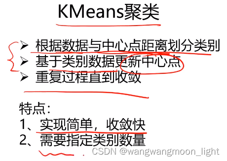

2.2 KMeans算法流程


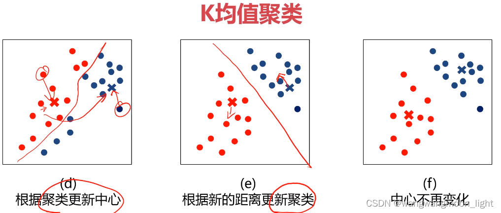
a) k == 2 分两类,随机选取聚类中心
b) 计算每个点都选取的聚类中心的距离
c d) 根据距离就划分好了两个类别,左上的红色部分离聚类中心红色近,右下的蓝色部分离聚类蓝色中心近
e) 更新聚类中心,并重新计算每个点到新的聚类中心的距离依此划分新的聚类
f) 直到中心点不再变化为止
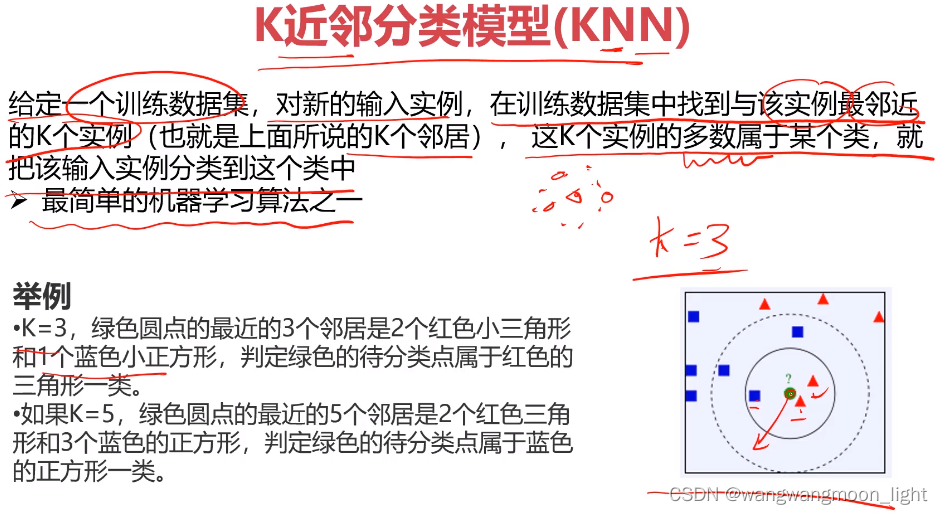
2.3 KNN – 监督学习
K近邻分类模型,给定一个训练数据集,对新的输入实例,在训练数据集中找到与该实例最邻近的K个实例,这K个实例的多数属于某个类,就是把该输入实例分类到这个类中
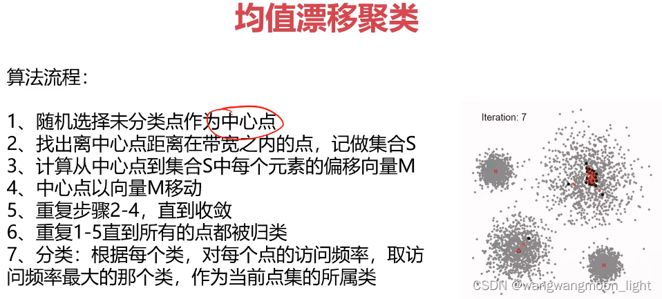
2.4 均值漂移聚类
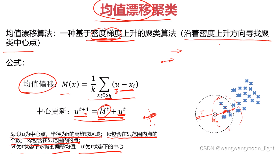
均值不断移动
3. 实战准备
任务:
1、采用Kmeans算法实现2D数据自动聚类,预测V1=80,V2=60数据类别;
2、计算预测准确率,完成结果矫正
3、采用KNN、Meanshift算法,重复步骤1-2
数据:data.csv
'''
任务:
1、**采用Kmeans算法实现2D数据自动聚类,预测V1=80,V2=60数据类别**;
2、计算预测准确率,完成结果矫正
3、采用KNN、Meanshift算法,重复步骤1-2
数据:data.csv
'''
#load the data
import pandas as pd
import numpy as np
from matplotlib import pyplot as plt
from sklearn.cluster import KMeans
data = pd.read_csv('data.csv')
data.head()
#define X and y
X = data.drop(['labels'],axis=1)
y = data.loc[:,'labels']
y.head()
pd.value_counts(y)
# %matplotlib inline
fig1 = plt.figure()
plt.scatter(X.loc[:,'V1'],X.loc[:,'V2'])
plt.title("un-labled data")
plt.xlabel('V1')
plt.ylabel('V2')
plt.show()
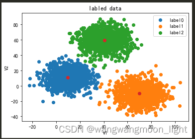
fig1 = plt.figure()
label0 = plt.scatter(X.loc[:,'V1'][y==0],X.loc[:,'V2'][y==0])
label1 = plt.scatter(X.loc[:,'V1'][y==1],X.loc[:,'V2'][y==1])
label2 = plt.scatter(X.loc[:,'V1'][y==2],X.loc[:,'V2'][y==2])
plt.title("labled data")
plt.xlabel('V1')
plt.ylabel('V2')
plt.legend((label0,label1,label2),('label0','label1','label2'))
plt.show()
#print(X.shape,y.shape)
# 1.KMeans
KM = KMeans(n_clusters=3,random_state=0)
KM.fit(X)
# 获取模型确定的中心点
centers = KM.cluster_centers_
fig3 = plt.figure()
label0 = plt.scatter(X.loc[:,'V1'][y==0],X.loc[:,'V2'][y==0])
label1 = plt.scatter(X.loc[:,'V1'][y==1],X.loc[:,'V2'][y==1])
label2 = plt.scatter(X.loc[:,'V1'][y==2],X.loc[:,'V2'][y==2])
plt.title("labled data")
plt.xlabel('V1')
plt.ylabel('V2')
plt.legend((label0,label1,label2),('label0','label1','label2'))
plt.scatter(centers[:,0],centers[:,1])
plt.show()
y_predict_test = KM.predict([[80,60]])
#print(y_predict_test)
y_predict = KM.predict(X)
#print(pd.value_counts(y_predict),pd.value_counts(y))
# 准确率计算
from sklearn.metrics import accuracy_score
accuracy = accuracy_score(y,y_predict)
print("accuracy", accuracy)
#visualize the data and results
fig4 = plt.subplot(121)
label0 = plt.scatter(X.loc[:,'V1'][y_predict==0],X.loc[:,'V2'][y_predict==0])
label1 = plt.scatter(X.loc[:,'V1'][y_predict==1],X.loc[:,'V2'][y_predict==1])
label2 = plt.scatter(X.loc[:,'V1'][y_predict==2],X.loc[:,'V2'][y_predict==2])
plt.title("predicted data")
plt.xlabel('V1')
plt.ylabel('V2')
plt.legend((label0,label1,label2),('label0','label1','label2'))
plt.scatter(centers[:,0],centers[:,1])
fig5 = plt.subplot(122)
label0 = plt.scatter(X.loc[:,'V1'][y==0],X.loc[:,'V2'][y==0])
label1 = plt.scatter(X.loc[:,'V1'][y==1],X.loc[:,'V2'][y==1])
label2 = plt.scatter(X.loc[:,'V1'][y==2],X.loc[:,'V2'][y==2])
plt.title("labled data")
plt.xlabel('V1')
plt.ylabel('V2')
plt.legend((label0,label1,label2),('label0','label1','label2'))
plt.scatter(centers[:,0],centers[:,1])
plt.show()
# 预测结果矫正
y_corrected = []
for i in y_predict:
if i==0:
y_corrected.append(1)
elif i==1:
y_corrected.append(2)
else:
y_corrected.append(0)
print(pd.value_counts(y_corrected),pd.value_counts(y))
print(accuracy_score(y,y_corrected))
y_corrected = np.array(y_corrected)
print(type(y_corrected))
fig6 = plt.subplot(121)
label0 = plt.scatter(X.loc[:,'V1'][y_corrected==0],X.loc[:,'V2'][y_corrected==0])
label1 = plt.scatter(X.loc[:,'V1'][y_corrected==1],X.loc[:,'V2'][y_corrected==1])
label2 = plt.scatter(X.loc[:,'V1'][y_corrected==2],X.loc[:,'V2'][y_corrected==2])
plt.title("corrected data")
plt.xlabel('V1')
plt.ylabel('V2')
plt.legend((label0,label1,label2),('label0','label1','label2'))
plt.scatter(centers[:,0],centers[:,1])
fig7 = plt.subplot(122)
label0 = plt.scatter(X.loc[:,'V1'][y==0],X.loc[:,'V2'][y==0])
label1 = plt.scatter(X.loc[:,'V1'][y==1],X.loc[:,'V2'][y==1])
label2 = plt.scatter(X.loc[:,'V1'][y==2],X.loc[:,'V2'][y==2])
plt.title("labled data")
plt.xlabel('V1')
plt.ylabel('V2')
plt.legend((label0,label1,label2),('label0','label1','label2'))
plt.scatter(centers[:,0],centers[:,1])
plt.show()
# 3.establish a KNN model
from sklearn.neighbors import KNeighborsClassifier
KNN = KNeighborsClassifier(n_neighbors=3)
KNN.fit(X,y)
#predict based on the test data V1=80, V2=60
y_predict_knn_test = KNN.predict([[80,60]])
y_predict_knn = KNN.predict(X)
print(y_predict_knn_test)
print('knn accuracy:',accuracy_score(y,y_predict_knn))
print(pd.value_counts(y_predict_knn),pd.value_counts(y))
fig6 = plt.subplot(121)
label0 = plt.scatter(X.loc[:,'V1'][y_predict_knn==0],X.loc[:,'V2'][y_predict_knn==0])
label1 = plt.scatter(X.loc[:,'V1'][y_predict_knn==1],X.loc[:,'V2'][y_predict_knn==1])
label2 = plt.scatter(X.loc[:,'V1'][y_predict_knn==2],X.loc[:,'V2'][y_predict_knn==2])
plt.title("knn results")
plt.xlabel('V1')
plt.ylabel('V2')
plt.legend((label0,label1,label2),('label0','label1','label2'))
plt.scatter(centers[:,0],centers[:,1])
fig7 = plt.subplot(122)
label0 = plt.scatter(X.loc[:,'V1'][y==0],X.loc[:,'V2'][y==0])
label1 = plt.scatter(X.loc[:,'V1'][y==1],X.loc[:,'V2'][y==1])
label2 = plt.scatter(X.loc[:,'V1'][y==2],X.loc[:,'V2'][y==2])
plt.title("labled data")
plt.xlabel('V1')
plt.ylabel('V2')
plt.legend((label0,label1,label2),('label0','label1','label2'))
plt.scatter(centers[:,0],centers[:,1])
plt.show()
from sklearn.cluster import MeanShift,estimate_bandwidth
#obtain the bandwidth 区域半径
bw = estimate_bandwidth(X,n_samples=500)
#print(bw)
# 3.establish the meanshift model-un-supervised model
ms = MeanShift(bandwidth=bw)
ms.fit(X)
y_predict_ms = ms.predict(X)
print(pd.value_counts(y_predict_ms),pd.value_counts(y))
print(centers)#kmeans聚类中心
#新增代码 打印使用meanshift算法获取的聚类中心 与kmeans算法对比 中心点非常接近
centers2 = ms.cluster_centers_
print(centers2)#meanshift聚类中心
fig6 = plt.subplot(121)
label0 = plt.scatter(X.loc[:,'V1'][y_predict_ms==0],X.loc[:,'V2'][y_predict_ms==0])
label1 = plt.scatter(X.loc[:,'V1'][y_predict_ms==1],X.loc[:,'V2'][y_predict_ms==1])
label2 = plt.scatter(X.loc[:,'V1'][y_predict_ms==2],X.loc[:,'V2'][y_predict_ms==2])
plt.title("ms results")
plt.xlabel('V1')
plt.ylabel('V2')
plt.legend((label0,label1,label2),('label0','label1','label2'))
plt.scatter(centers[:,0],centers[:,1])
fig7 = plt.subplot(122)
label0 = plt.scatter(X.loc[:,'V1'][y==0],X.loc[:,'V2'][y==0])
label1 = plt.scatter(X.loc[:,'V1'][y==1],X.loc[:,'V2'][y==1])
label2 = plt.scatter(X.loc[:,'V1'][y==2],X.loc[:,'V2'][y==2])
plt.title("labled data")
plt.xlabel('V1')
plt.ylabel('V2')
plt.legend((label0,label1,label2),('label0','label1','label2'))
plt.scatter(centers[:,0],centers[:,1])
plt.show()
#correct the results
y_corrected_ms = []
for i in y_predict_ms:
if i==0:
y_corrected_ms.append(2)
elif i==1:
y_corrected_ms.append(1)
else:
y_corrected_ms.append(0)
print(pd.value_counts(y_corrected_ms),pd.value_counts(y))
#convert the results to numpy array
y_corrected_ms = np.array(y_corrected_ms)
print(type(y_corrected_ms))
fig6 = plt.subplot(121)
label0 = plt.scatter(X.loc[:,'V1'][y_corrected_ms==0],X.loc[:,'V2'][y_corrected_ms==0])
label1 = plt.scatter(X.loc[:,'V1'][y_corrected_ms==1],X.loc[:,'V2'][y_corrected_ms==1])
label2 = plt.scatter(X.loc[:,'V1'][y_corrected_ms==2],X.loc[:,'V2'][y_corrected_ms==2])
plt.title("ms corrected results")
plt.xlabel('V1')
plt.ylabel('V2')
plt.legend((label0,label1,label2),('label0','label1','label2'))
plt.scatter(centers[:,0],centers[:,1])
fig7 = plt.subplot(122)
label0 = plt.scatter(X.loc[:,'V1'][y==0],X.loc[:,'V2'][y==0])
label1 = plt.scatter(X.loc[:,'V1'][y==1],X.loc[:,'V2'][y==1])
label2 = plt.scatter(X.loc[:,'V1'][y==2],X.loc[:,'V2'][y==2])
plt.title("labled data")
plt.xlabel('V1')
plt.ylabel('V2')
plt.legend((label0,label1,label2),('label0','label1','label2'))
plt.scatter(centers[:,0],centers[:,1])
plt.show()
[80,60] result[2] label2
在实际中分类后需要矫正数据,如上代码有矫正数据的过程。