Matlab: Introduction to Hybrid Beamforming

文章目录

来源
混合波束赋形的基本概念
System Setup

来源

在matlab的命令行输入
doc hybrid beamforming

混合波束赋形的基本概念

混合波束形成简介
本例介绍了混合波束形成的基本概念，并说明了如何模拟这种系统。

现代无线通信系统使用空间复用来提高散射体丰富的环境中系统内的数据吞吐量。为了通过信道发送多个数据流，从信道矩阵中导出一组预编码和组合权重。那么每个数据流都可以独立恢复。这些权重包含幅度和相位项，通常应用于数字域。模拟这种系统的一个例子可以在使用天线阵列提高无线通信的SNR和容量的例子中找到。在下图所示的系统图中，每个天线都连接到一个独特的发射和接收（TR）模块。在这里插入图片描述

对高数据速率和更多用户容量的日益增长的需求增加了更有效地使用频谱的需求。因此，下一代5G无线系统将使用毫米波频段来利用其更宽的带宽。此外，5G系统部署了大规模天线阵列，以减轻毫米波频段的严重传播损耗。然而，这些配置带来了其独特的技术挑战。

与目前的无线系统相比，毫米波波段的波长要小得多。虽然这允许一个阵列包含更多具有相同物理尺寸的单元，但为每个天线单元提供一个TR模块会变得昂贵得多。因此，作为一种折衷，TR开关通常用于为多个天线元件供电。这与雷达社区中使用的子阵列配置是相同的概念。下图显示了一种这样的配置。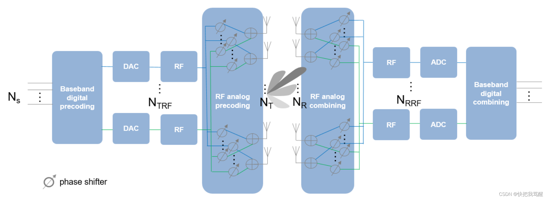在这里插入图片描述
上图显示，在发射端，TR开关的数量小于天线单元的数量 $N_T$ 。为了提供更大的灵活性，每个天线元件可以连接到一个或多个TR模块。此外，可以在每个TR模块和天线之间插入模拟移相器，以提供一些有限的转向能力。

接收器端的配置类似，如图所示。此系统可以支持的最大数据流数量 $N_S$ 是 $N_{TRF}$ 和 $N_{RRF}$ 中较小的一个。

在这种配置中，不再可能对每个天线元件应用数字权重。相反，数字权重只能应用于每个RF链。在元件级，信号由模拟移相器调整，该移相器仅改变信号的相位。因此，预编码或组合实际上分两个阶段完成。由于这种方法在数字域和模拟域都执行波束成形，因此被称为混合波束成形。

System Setup

This section simulates a 64 x 16 MIMO hybrid beamforming system, with a 64-element square array with 4 RF chains on the transmitter side and a 16-element square array with 4 RF chains on the receiver side.

Nt = 64;
NtRF = 4;

Nr = 16;
NrRF = 4;

In this simulation, it is assumed that each antenna is connected to all RF chains. Thus, each antenna is connected to 4 phase shifters. Such an array can be modeled by partitioning the array aperture into 4 completely connected subarrays.

rng(4096);
c = 3e8;
fc = 28e9;
lambda = c/fc;
txarray = phased.PartitionedArray(...
    'Array',phased.URA([sqrt(Nt) sqrt(Nt)],lambda/2),...
    'SubarraySelection',ones(NtRF,Nt),'SubarraySteering','Custom');
rxarray = phased.PartitionedArray(...
    'Array',phased.URA([sqrt(Nr) sqrt(Nr)],lambda/2),...
    'SubarraySelection',ones(NrRF,Nr),'SubarraySteering','Custom');

To maximize the spectral efficiency, each RF chain can be used to send an independent data stream. In this case, the system can support up to 4 streams.

Next, assume a scattering environment with 6 scattering clusters randomly distributed in space. Within each cluster, there are 8 closely located scatterers with an angle spread of 5 degrees, for a total of 48 scatterers. The path gain for each scatterer is obtained from a complex circular symmetric Gaussian distribution.

Ncl = 6;
Nray = 8;
Nscatter = Nray*Ncl;
angspread = 5;
% compute randomly placed scatterer clusters
txclang = [rand(1,Ncl)*120-60;rand(1,Ncl)*60-30];
rxclang = [rand(1,Ncl)*120-60;rand(1,Ncl)*60-30];
txang = zeros(2,Nscatter);
rxang = zeros(2,Nscatter);
% compute the rays within each cluster
for m = 1:Ncl
    txang(:,(m-1)*Nray+(1:Nray)) = randn(2,Nray)*sqrt(angspread)+txclang(:,m);
    rxang(:,(m-1)*Nray+(1:Nray)) = randn(2,Nray)*sqrt(angspread)+rxclang(:,m);
end

g = (randn(1,Nscatter)+1i*randn(1,Nscatter))/sqrt(Nscatter);

The channel matrix can be formed as 
txpos = getElementPosition(txarray)/lambda;
rxpos = getElementPosition(rxarray)/lambda;
H = scatteringchanmtx(txpos,rxpos,txang,rxang,g);

Hybrid Weights Computation
In a spatial multiplexing system with all digital beamforming, the signal is modulated by a set of precoding weights, propagated through the channel, and recovered by a set of combining weights. Mathematically, this process can be described by Y = (XFH+N)W where X is an Ns-column matrix whose columns are data streams, F is an Ns Nt matrix representing the precoding weights, W is an Nr Ns matrix representing the combining weights, N is an Nr-column matrix whose columns are the receiver noise at each element, and Y is an Ns-column matrix whose columns are recovered data streams. Since the goal of the system is to achieve better spectral efficiency, obtaining the precoding and combining weights can be considered as an optimization problem where the optimal precoding and combining weights make the product of FHW’ a diagonal matrix so each data stream can be recovered independently.
In a hybrid beamforming system, the signal flow is similar. Both the precoding weights and the combining weights are combinations of baseband digital weights and RF band analog weights. The baseband digital weights convert the incoming data streams to input signals at each RF chain and the analog weights then convert the signal at each RF chain to the signal radiated or collected at each antenna element. Note that the analog weights can only contain phase shifts.
Mathematically, it can be written as F=FbbFrf and W=WbbWrf, where Fbb is an Ns NtRF matrix, Frf an NtRF Nt matrix, Wbb an NrRF Ns matrix, and Wrf an Nr NrRF matrix. Since both Frf and Wrf can only be used to modify the signal phase, there are extra constraints in the optimization process to identify the optimal precoding and combining weights. Ideally, the resulting combination of FbbFrf and Wrf*Wbb are close approximations of F and W that are obtained without those constraints.
Unfortunately, optimizing all four matrix variables simultaneously is quite difficult. Therefore, many algorithms are proposed to arrive at suboptimal weights with a reasonable computational load. This example uses the approach proposed in [1] which decouples the optimizations for the precoding and combining weights. It first uses the orthogonal matching pursuit algorithm to derive the precoding weights. Once the precoding weights are computed, the result is then used to obtain the corresponding combining weights.
Assuming the channel is known, the unconstrained optimal precoding weights can be obtained by diagonalizing the channel matrix and extracting the first NtRF dominating modes. The transmit beam pattern can be plotted as

F = diagbfweights(H);
F = F(1:NtRF,:);
pattern(txarray,fc,-90:90,-90:90,'Type','efield',...
    'ElementWeights',F','PropagationSpeed',c);

The response pattern above shows that even in a multipath environment, there are limited number of dominant directions.
The hybrid weights, on the other hand, can be computed as

At = steervec(txpos,txang);
Ar = steervec(rxpos,rxang);

Ns = NtRF;
[Fbb,Frf] = omphybweights(H,Ns,NtRF,At);

The beam pattern of the hybrid weights is shown below:

pattern(txarray,fc,-90:90,-90:90,'Type','efield',...
    'ElementWeights',Frf'*Fbb','PropagationSpeed',c);

Compared to the beam pattern obtained using the optimal weights, the beam pattern using the hybrid weights is similar, especially for dominant beams. This means that the data streams can be successfully transmitted through those beams using hybrid weights.

Spectral Efficiency Comparison
One of the system level performance metrics of a 5G system is the spectral efficiency. The next section compares the spectral efficiency achieved using the optimal weights with that of the proposed hybrid beamforming weights. The simulation assumes 1 or 2 data streams as outlined in [1]. The transmit antenna array is assumed to be at a base station, with a focused beamwidth of 60 degrees in azimuth and 20 degrees in elevation. The signal can arrive at the receive array from any direction. The resulting spectral efficiency curve is obtained from 50 Monte-Carlo trials for each SNR.

snr_param = -40:5:0;
Nsnr = numel(snr_param);
Ns_param = [1 2];
NNs = numel(Ns_param);

NtRF = 4;
NrRF = 4;

Ropt = zeros(Nsnr,NNs);
Rhyb = zeros(Nsnr,NNs);
Niter = 50;

for m = 1:Nsnr
    snr = db2pow(snr_param(m));
    for n = 1:Niter
        % Channel realization
        txang = [rand(1,Nscatter)*60-30;rand(1,Nscatter)*20-10];
        rxang = [rand(1,Nscatter)*180-90;rand(1,Nscatter)*90-45];
        At = steervec(txpos,txang);
        Ar = steervec(rxpos,rxang);
        g = (randn(1,Nscatter)+1i*randn(1,Nscatter))/sqrt(Nscatter);
        H = scatteringchanmtx(txpos,rxpos,txang,rxang,g);
        
        for k = 1:NNs
            Ns = Ns_param(k);
            % Compute optimal weights and its spectral efficiency
            [Fopt,Wopt] = helperOptimalHybridWeights(H,Ns,1/snr);
            Ropt(m,k) = Ropt(m,k)+helperComputeSpectralEfficiency(H,Fopt,Wopt,Ns,snr);

            % Compute hybrid weights and its spectral efficiency
            [Fbb,Frf,Wbb,Wrf] = omphybweights(H,Ns,NtRF,At,NrRF,Ar,1/snr);
            Rhyb(m,k) = Rhyb(m,k)+helperComputeSpectralEfficiency(H,Fbb*Frf,Wrf*Wbb,Ns,snr);
        end
    end
end
Ropt = Ropt/Niter;
Rhyb = Rhyb/Niter;

plot(snr_param,Ropt(:,1),'--sr',...
    snr_param,Ropt(:,2),'--b',...
    snr_param,Rhyb(:,1),'-sr',...
    snr_param,Rhyb(:,2),'-b');
xlabel('SNR (dB)');
ylabel('Spectral Efficiency (bits/s/Hz');
legend('Ns=1 optimal','Ns=2 optimal','Ns=1 hybrid', 'Ns=2 hybrid',...
    'Location','best');
grid on;

在这里插入图片描述

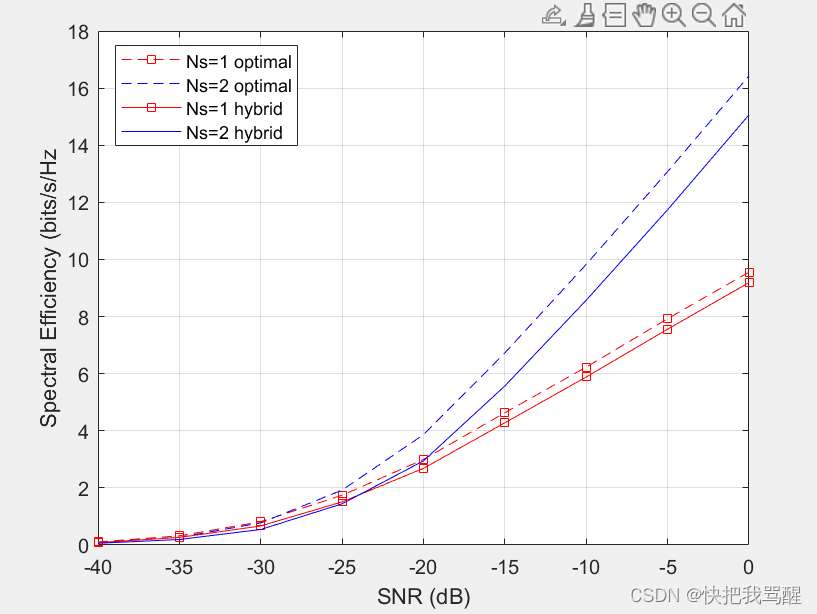
This figure shows that the spectral efficiency improves significantly when we increase the number of data streams. In addition, the hybrid beamforming can perform close to what optimal weights can offer using less hardware.

Summary
This example introduces the basic concept of hybrid beamforming and shows how to split the precoding and combining weights using orthogonal matching pursuit algorithm. It shows that hybrid beamforming can closely match the performance offered by optimal digital weights.
References
[1] Omar El Ayach, et al. Spatially Sparse Precoding in Millimeter wave MIMO Systems, IEEE Transactions on Wireless Communications, Vol. 13, No. 3, March 2014.
Copyright 2017 The MathWorks, Inc.