PyTorch 2.2 中文官方教程（一）

PyTorch 秘籍

原文：pytorch.org/tutorials/recipes/recipes_index.html

译者：飞龙

协议：CC BY-NC-SA 4.0

秘籍是关于如何使用特定 PyTorch 功能的简短、可操作的示例，与我们的全长教程不同。

PyTorch 原型示例

原文：pytorch.org/tutorials/prototype/prototype_index.html

译者：飞龙

协议：CC BY-NC-SA 4.0

原型功能不作为二进制分发的一部分，比如 PyPI 或 Conda（除非可能在运行时标志后面）。为了测试这些功能，我们会根据功能的不同，建议从主分支构建或使用在pytorch.org上提供的夜间版本。

承诺水平：我们承诺只收集关于这些功能的高带宽反馈。基于这些反馈和社区成员之间的潜在进一步互动，作为一个社区，我们将决定是否要升级承诺水平或快速失败。

PyTorch 介绍

学习基础知识

原文：pytorch.org/tutorials/beginner/basics/intro.html

译者：飞龙

协议：CC BY-NC-SA 4.0

注意

点击这里下载完整示例代码

学习基础知识 || 快速入门 || 张量 || 数据集和数据加载器 || 转换 || 构建模型 || 自动微分 || 优化 || 保存和加载模型

作者：Suraj Subramanian、Seth Juarez、Cassie Breviu、Dmitry Soshnikov、Ari Bornstein

大多数机器学习工作流程涉及处理数据、创建模型、优化模型参数和保存训练好的模型。本教程向您介绍了在 PyTorch 中实现的完整 ML 工作流程，并提供了有关这些概念的更多学习链接。

我们将使用 FashionMNIST 数据集训练一个神经网络，该神经网络可以预测输入图像是否属于以下类别之一：T 恤/上衣、裤子、套头衫、连衣裙、外套、凉鞋、衬衫、运动鞋、包或短靴。

本教程假定您对 Python 和深度学习概念有基本了解。

运行教程代码

您可以通过以下几种方式运行本教程：

在云端：这是开始的最简单方式！每个部分顶部都有一个“在 Microsoft Learn 中运行”和“在 Google Colab 中运行”的链接，分别在 Microsoft Learn 或 Google Colab 中打开一个集成的笔记本，其中包含完全托管环境中的代码。
本地运行：此选项要求您首先在本地计算机上设置 PyTorch 和 TorchVision（安装说明）。下载笔记本或将代码复制到您喜欢的 IDE 中。

如何使用本指南

如果您熟悉其他深度学习框架，请先查看 0. 快速入门，快速熟悉 PyTorch 的 API。

如果您是深度学习框架的新手，请直接进入我们逐步指南的第一部分：1. 张量。

快速入门 1. 张量 2. 数据集和数据加载器 3. 转换 4. 构建模型 5. 自动微分 6. 优化循环 7. 保存、加载和使用模型

脚本的总运行时间：（0 分钟 0.000 秒）

下载 Python 源代码：intro.py

下载 Jupyter 笔记本：intro.ipynb

Sphinx-Gallery 生成的图库

快速入门

原文：pytorch.org/tutorials/beginner/basics/quickstart_tutorial.html

译者：飞龙

协议：CC BY-NC-SA 4.0

注意

点击这里下载完整示例代码

学习基础知识 || 快速入门 || 张量 || 数据集和数据加载器 || 转换 || 构建模型 || 自动求导 || 优化 || 保存和加载模型

本节介绍了机器学习中常见任务的 API。请参考每个部分中的链接以深入了解。

处理数据

PyTorch 有两个用于处理数据的基本方法：torch.utils.data.DataLoader和torch.utils.data.Dataset。Dataset存储样本及其对应的标签，而DataLoader将一个可迭代对象包装在Dataset周围。

import torch
from torch import nn
from torch.utils.data import DataLoader
from torchvision import datasets
from torchvision.transforms import ToTensor

PyTorch 提供了领域特定的库，如TorchText、TorchVision和TorchAudio，其中包括数据集。在本教程中，我们将使用一个 TorchVision 数据集。

torchvision.datasets模块包含许多现实世界视觉数据的Dataset对象，如 CIFAR、COCO（完整列表在此）。在本教程中，我们使用 FashionMNIST 数据集。每个 TorchVision Dataset都包括两个参数：transform和target_transform，分别用于修改样本和标签。

# Download training data from open datasets.
training_data = datasets.FashionMNIST(
    root="data",
    train=True,
    download=True,
    transform=ToTensor(),
)

# Download test data from open datasets.
test_data = datasets.FashionMNIST(
    root="data",
    train=False,
    download=True,
    transform=ToTensor(),
)

Downloading http://fashion-mnist.s3-website.eu-central-1.amazonaws.com/train-images-idx3-ubyte.gz
Downloading http://fashion-mnist.s3-website.eu-central-1.amazonaws.com/train-images-idx3-ubyte.gz to data/FashionMNIST/raw/train-images-idx3-ubyte.gz

  0%|          | 0/26421880 [00:00<?, ?it/s]
  0%|          | 65536/26421880 [00:00<01:12, 362268.71it/s]
  1%|          | 229376/26421880 [00:00<00:38, 680481.08it/s]
  3%|3         | 819200/26421880 [00:00<00:13, 1853717.26it/s]
 11%|#1        | 3014656/26421880 [00:00<00:03, 7167253.78it/s]
 24%|##3       | 6258688/26421880 [00:00<00:01, 11757636.19it/s]
 42%|####1     | 11075584/26421880 [00:00<00:00, 20718315.26it/s]
 55%|#####4    | 14483456/26421880 [00:01<00:00, 20324854.10it/s]
 74%|#######4  | 19562496/26421880 [00:01<00:00, 27572084.42it/s]
 87%|########7 | 23068672/26421880 [00:01<00:00, 27527140.28it/s]
100%|#########9| 26312704/26421880 [00:01<00:00, 26297445.36it/s]
100%|##########| 26421880/26421880 [00:01<00:00, 18147607.68it/s]
Extracting data/FashionMNIST/raw/train-images-idx3-ubyte.gz to data/FashionMNIST/raw

Downloading http://fashion-mnist.s3-website.eu-central-1.amazonaws.com/train-labels-idx1-ubyte.gz
Downloading http://fashion-mnist.s3-website.eu-central-1.amazonaws.com/train-labels-idx1-ubyte.gz to data/FashionMNIST/raw/train-labels-idx1-ubyte.gz

  0%|          | 0/29515 [00:00<?, ?it/s]
100%|##########| 29515/29515 [00:00<00:00, 327172.52it/s]
Extracting data/FashionMNIST/raw/train-labels-idx1-ubyte.gz to data/FashionMNIST/raw

Downloading http://fashion-mnist.s3-website.eu-central-1.amazonaws.com/t10k-images-idx3-ubyte.gz
Downloading http://fashion-mnist.s3-website.eu-central-1.amazonaws.com/t10k-images-idx3-ubyte.gz to data/FashionMNIST/raw/t10k-images-idx3-ubyte.gz

  0%|          | 0/4422102 [00:00<?, ?it/s]
  1%|1         | 65536/4422102 [00:00<00:11, 363567.22it/s]
  5%|5         | 229376/4422102 [00:00<00:06, 694276.06it/s]
 19%|#9        | 851968/4422102 [00:00<00:01, 1962897.43it/s]
 64%|######3   | 2818048/4422102 [00:00<00:00, 5508389.41it/s]
100%|##########| 4422102/4422102 [00:00<00:00, 6087122.93it/s]
Extracting data/FashionMNIST/raw/t10k-images-idx3-ubyte.gz to data/FashionMNIST/raw

Downloading http://fashion-mnist.s3-website.eu-central-1.amazonaws.com/t10k-labels-idx1-ubyte.gz
Downloading http://fashion-mnist.s3-website.eu-central-1.amazonaws.com/t10k-labels-idx1-ubyte.gz to data/FashionMNIST/raw/t10k-labels-idx1-ubyte.gz

  0%|          | 0/5148 [00:00<?, ?it/s]
100%|##########| 5148/5148 [00:00<00:00, 36228652.67it/s]
Extracting data/FashionMNIST/raw/t10k-labels-idx1-ubyte.gz to data/FashionMNIST/raw

我们将Dataset作为参数传递给DataLoader。这会将一个可迭代对象包装在我们的数据集周围，并支持自动批处理、采样、洗牌和多进程数据加载。在这里，我们定义了一个批量大小为 64，即数据加载器可迭代对象中的每个元素将返回一个包含 64 个特征和标签的批次。

batch_size = 64

# Create data loaders.
train_dataloader = DataLoader(training_data, batch_size=batch_size)
test_dataloader = DataLoader(test_data, batch_size=batch_size)

for X, y in test_dataloader:
    print(f"Shape of X [N, C, H, W]: {X.shape}")
    print(f"Shape of y: {y.shape}  {y.dtype}")
    break

Shape of X [N, C, H, W]: torch.Size([64, 1, 28, 28])
Shape of y: torch.Size([64]) torch.int64

关于在 PyTorch 中加载数据。

创建模型

要在 PyTorch 中定义神经网络，我们创建一个从nn.Module继承的类。我们在__init__函数中定义网络的层，并在forward函数中指定数据如何通过网络传递。为了加速神经网络中的操作，我们将其移动到 GPU 或 MPS（如果可用）。

# Get cpu, gpu or mps device for training.
device = (
    "cuda"
    if torch.cuda.is_available()
    else "mps"
    if torch.backends.mps.is_available()
    else "cpu"
)
print(f"Using {device} device")

# Define model
class NeuralNetwork(nn.Module):
    def __init__(self):
        super().__init__()
        self.flatten = nn.Flatten()
        self.linear_relu_stack = nn.Sequential(
            nn.Linear(28*28, 512),
            nn.ReLU(),
            nn.Linear(512, 512),
            nn.ReLU(),
            nn.Linear(512, 10)
        )

    def forward(self, x):
        x = self.flatten(x)
        logits = self.linear_relu_stack(x)
        return logits

model = NeuralNetwork().to(device)
print(model)

Using cuda device
NeuralNetwork(
  (flatten): Flatten(start_dim=1, end_dim=-1)
  (linear_relu_stack): Sequential(
    (0): Linear(in_features=784, out_features=512, bias=True)
    (1): ReLU()
    (2): Linear(in_features=512, out_features=512, bias=True)
    (3): ReLU()
    (4): Linear(in_features=512, out_features=10, bias=True)
  )
)

关于在 PyTorch 中构建神经网络。

优化模型参数

要训练一个模型，我们需要一个损失函数和一个优化器。

loss_fn = nn.CrossEntropyLoss()
optimizer = torch.optim.SGD(model.parameters(), lr=1e-3)

在单个训练循环中，模型对训练数据集进行预测（以批量方式提供），并将预测错误反向传播以调整模型的参数。

def train(dataloader, model, loss_fn, optimizer):
    size = len(dataloader.dataset)
    model.train()
    for batch, (X, y) in enumerate(dataloader):
        X, y = X.to(device), y.to(device)

        # Compute prediction error
        pred = model(X)
        loss = loss_fn(pred, y)

        # Backpropagation
        loss.backward()
        optimizer.step()
        optimizer.zero_grad()

        if batch % 100 == 0:
            loss, current = loss.item(), (batch + 1) * len(X)
            print(f"loss: {loss:>7f} [{current:>5d}/{size:>5d}]")

我们还会检查模型在测试数据集上的表现，以确保它正在学习。

def test(dataloader, model, loss_fn):
    size = len(dataloader.dataset)
    num_batches = len(dataloader)
    model.eval()
    test_loss, correct = 0, 0
    with torch.no_grad():
        for X, y in dataloader:
            X, y = X.to(device), y.to(device)
            pred = model(X)
            test_loss += loss_fn(pred, y).item()
            correct += (pred.argmax(1) == y).type(torch.float).sum().item()
    test_loss /= num_batches
    correct /= size
    print(f"Test Error: \n Accuracy: {(100*correct):>0.1f}%, Avg loss: {test_loss:>8f}  \n")

训练过程是在几个迭代（epochs）中进行的。在每个迭代中，模型学习参数以做出更好的预测。我们在每个迭代中打印模型的准确性和损失；我们希望看到准确性随着每个迭代的增加而增加，损失随着每个迭代的减少而减少。

epochs = 5
for t in range(epochs):
    print(f"Epoch {t+1}\n-------------------------------")
    train(train_dataloader, model, loss_fn, optimizer)
    test(test_dataloader, model, loss_fn)
print("Done!")

Epoch 1
-------------------------------
loss: 2.303494  [   64/60000]
loss: 2.294637  [ 6464/60000]
loss: 2.277102  [12864/60000]
loss: 2.269977  [19264/60000]
loss: 2.254235  [25664/60000]
loss: 2.237146  [32064/60000]
loss: 2.231055  [38464/60000]
loss: 2.205037  [44864/60000]
loss: 2.203240  [51264/60000]
loss: 2.170889  [57664/60000]
Test Error:
 Accuracy: 53.9%, Avg loss: 2.168588

Epoch 2
-------------------------------
loss: 2.177787  [   64/60000]
loss: 2.168083  [ 6464/60000]
loss: 2.114910  [12864/60000]
loss: 2.130412  [19264/60000]
loss: 2.087473  [25664/60000]
loss: 2.039670  [32064/60000]
loss: 2.054274  [38464/60000]
loss: 1.985457  [44864/60000]
loss: 1.996023  [51264/60000]
loss: 1.917241  [57664/60000]
Test Error:
 Accuracy: 60.2%, Avg loss: 1.920374

Epoch 3
-------------------------------
loss: 1.951705  [   64/60000]
loss: 1.919516  [ 6464/60000]
loss: 1.808730  [12864/60000]
loss: 1.846550  [19264/60000]
loss: 1.740618  [25664/60000]
loss: 1.698733  [32064/60000]
loss: 1.708889  [38464/60000]
loss: 1.614436  [44864/60000]
loss: 1.646475  [51264/60000]
loss: 1.524308  [57664/60000]
Test Error:
 Accuracy: 61.4%, Avg loss: 1.547092

Epoch 4
-------------------------------
loss: 1.612695  [   64/60000]
loss: 1.570870  [ 6464/60000]
loss: 1.424730  [12864/60000]
loss: 1.489542  [19264/60000]
loss: 1.367256  [25664/60000]
loss: 1.373464  [32064/60000]
loss: 1.376744  [38464/60000]
loss: 1.304962  [44864/60000]
loss: 1.347154  [51264/60000]
loss: 1.230661  [57664/60000]
Test Error:
 Accuracy: 62.7%, Avg loss: 1.260891

Epoch 5
-------------------------------
loss: 1.337803  [   64/60000]
loss: 1.313278  [ 6464/60000]
loss: 1.151837  [12864/60000]
loss: 1.252142  [19264/60000]
loss: 1.123048  [25664/60000]
loss: 1.159531  [32064/60000]
loss: 1.175011  [38464/60000]
loss: 1.115554  [44864/60000]
loss: 1.160974  [51264/60000]
loss: 1.062730  [57664/60000]
Test Error:
 Accuracy: 64.6%, Avg loss: 1.087374

Done!

关于训练模型。

保存模型

保存模型的常见方法是序列化内部状态字典（包含模型参数）。

torch.save(model.state_dict(), "model.pth")
print("Saved PyTorch Model State to model.pth")

Saved PyTorch Model State to model.pth

加载模型

加载模型的过程包括重新创建模型结构并将状态字典加载到其中。

model = NeuralNetwork().to(device)
model.load_state_dict(torch.load("model.pth"))

<All keys matched successfully>

现在可以使用这个模型进行预测了。

classes = [
    "T-shirt/top",
    "Trouser",
    "Pullover",
    "Dress",
    "Coat",
    "Sandal",
    "Shirt",
    "Sneaker",
    "Bag",
    "Ankle boot",
]

model.eval()
x, y = test_data[0][0], test_data[0][1]
with torch.no_grad():
    x = x.to(device)
    pred = model(x)
    predicted, actual = classes[pred[0].argmax(0)], classes[y]
    print(f'Predicted: "{predicted}", Actual: "{actual}"')

Predicted: "Ankle boot", Actual: "Ankle boot"

关于保存和加载模型。

脚本的总运行时间：（0 分钟 58.630 秒）

下载 Python 源代码：quickstart_tutorial.py

下载 Jupyter 笔记本：quickstart_tutorial.ipynb

Sphinx-Gallery 生成的图库

张量

原文：pytorch.org/tutorials/beginner/basics/tensorqs_tutorial.html

译者：飞龙

协议：CC BY-NC-SA 4.0

注意

点击这里下载完整示例代码

学习基础知识 || 快速入门 || 张量 || 数据集和数据加载器 || 变换 || 构建模型 || 自动微分 || 优化 || 保存和加载模型

张量是一种类似于数组和矩阵的专门数据结构。在 PyTorch 中，我们使用张量来编码模型的输入和输出，以及模型的参数。

张量类似于NumPy 的 ndarrays，不同之处在于张量可以在 GPU 或其他硬件加速器上运行。实际上，张量和 NumPy 数组通常可以共享相同的基础内存，消除了复制数据的需要（请参阅与 NumPy 的桥接）。张量还针对自动微分进行了优化（我们稍后将在自动微分部分看到更多）。如果您熟悉 ndarrays，您将很容易使用张量 API。如果不熟悉，请跟着学习！

import torch
import numpy as np

初始化张量

张量可以以各种方式初始化。看看以下示例：

直接从数据中

可以直接从数据创建张量。数据类型会自动推断。

data = [[1, 2],[3, 4]]
x_data = torch.tensor(data)

从 NumPy 数组

可以从 NumPy 数组创建张量（反之亦然-请参阅与 NumPy 的桥接）。

np_array = np.array(data)
x_np = torch.from_numpy(np_array)

从另一个张量中：

新张量保留了参数张量的属性（形状、数据类型），除非显式覆盖。

x_ones = torch.ones_like(x_data) # retains the properties of x_data
print(f"Ones Tensor: \n  {x_ones}  \n")

x_rand = torch.rand_like(x_data, dtype=torch.float) # overrides the datatype of x_data
print(f"Random Tensor: \n  {x_rand}  \n")

Ones Tensor:
 tensor([[1, 1],
        [1, 1]])

Random Tensor:
 tensor([[0.8823, 0.9150],
        [0.3829, 0.9593]])

使用随机或常量值：

shape是张量维度的元组。在下面的函数中，它确定输出张量的维度。

shape = (2,3,)
rand_tensor = torch.rand(shape)
ones_tensor = torch.ones(shape)
zeros_tensor = torch.zeros(shape)

print(f"Random Tensor: \n  {rand_tensor}  \n")
print(f"Ones Tensor: \n  {ones_tensor}  \n")
print(f"Zeros Tensor: \n  {zeros_tensor}")

Random Tensor:
 tensor([[0.3904, 0.6009, 0.2566],
        [0.7936, 0.9408, 0.1332]])

Ones Tensor:
 tensor([[1., 1., 1.],
        [1., 1., 1.]])

Zeros Tensor:
 tensor([[0., 0., 0.],
        [0., 0., 0.]])

张量的属性

张量属性描述了它们的形状、数据类型和存储它们的设备。

tensor = torch.rand(3,4)

print(f"Shape of tensor: {tensor.shape}")
print(f"Datatype of tensor: {tensor.dtype}")
print(f"Device tensor is stored on: {tensor.device}")

Shape of tensor: torch.Size([3, 4])
Datatype of tensor: torch.float32
Device tensor is stored on: cpu

张量上的操作

包括算术、线性代数、矩阵操作（转置、索引、切片）、采样等在内的 100 多个张量操作在这里得到了全面描述。

这些操作中的每一个都可以在 GPU 上运行（通常比在 CPU 上速度更快）。如果您在使用 Colab，请转到运行时 > 更改运行时类型 > GPU 来分配 GPU。

默认情况下，张量在 CPU 上创建。我们需要使用.to方法显式将张量移动到 GPU（在检查 GPU 可用性后）。请记住，在设备之间复制大型张量可能会在时间和内存方面昂贵！

# We move our tensor to the GPU if available
if torch.cuda.is_available():
    tensor = tensor.to("cuda")

尝试运行列表中的一些操作。如果您熟悉 NumPy API，您会发现 Tensor API 非常易于使用。

标准类似于 numpy 的索引和切片：

tensor = torch.ones(4, 4)
print(f"First row: {tensor[0]}")
print(f"First column: {tensor[:,  0]}")
print(f"Last column: {tensor[...,  -1]}")
tensor[:,1] = 0
print(tensor)

First row: tensor([1., 1., 1., 1.])
First column: tensor([1., 1., 1., 1.])
Last column: tensor([1., 1., 1., 1.])
tensor([[1., 0., 1., 1.],
        [1., 0., 1., 1.],
        [1., 0., 1., 1.],
        [1., 0., 1., 1.]])

连接张量 您可以使用torch.cat沿着给定维度连接一系列张量。另请参阅torch.stack，另一个微妙不同于torch.cat的张量连接运算符。

t1 = torch.cat([tensor, tensor, tensor], dim=1)
print(t1)

tensor([[1., 0., 1., 1., 1., 0., 1., 1., 1., 0., 1., 1.],
        [1., 0., 1., 1., 1., 0., 1., 1., 1., 0., 1., 1.],
        [1., 0., 1., 1., 1., 0., 1., 1., 1., 0., 1., 1.],
        [1., 0., 1., 1., 1., 0., 1., 1., 1., 0., 1., 1.]])

算术操作

# This computes the matrix multiplication between two tensors. y1, y2, y3 will have the same value
# ``tensor.T`` returns the transpose of a tensor
y1 = tensor @ tensor.T
y2 = tensor.matmul(tensor.T)

y3 = torch.rand_like(y1)
torch.matmul(tensor, tensor.T, out=y3)

# This computes the element-wise product. z1, z2, z3 will have the same value
z1 = tensor * tensor
z2 = tensor.mul(tensor)

z3 = torch.rand_like(tensor)
torch.mul(tensor, tensor, out=z3)

tensor([[1., 0., 1., 1.],
        [1., 0., 1., 1.],
        [1., 0., 1., 1.],
        [1., 0., 1., 1.]])

单元素张量 如果您有一个单元素张量，例如通过将张量的所有值聚合为一个值，您可以使用item()将其转换为 Python 数值：

agg = tensor.sum()
agg_item = agg.item()
print(agg_item, type(agg_item))

12.0 <class 'float'>

原地操作 将结果存储到操作数中的操作称为原地操作。它们以_后缀表示。例如：x.copy_(y)，x.t_()，将改变x。

print(f"{tensor}  \n")
tensor.add_(5)
print(tensor)

tensor([[1., 0., 1., 1.],
        [1., 0., 1., 1.],
        [1., 0., 1., 1.],
        [1., 0., 1., 1.]])

tensor([[6., 5., 6., 6.],
        [6., 5., 6., 6.],
        [6., 5., 6., 6.],
        [6., 5., 6., 6.]])

注意

原地操作可以节省一些内存，但在计算导数时可能会出现问题，因为会立即丢失历史记录。因此，不建议使用它们。

与 NumPy 的桥接

CPU 上的张量和 NumPy 数组可以共享它们的基础内存位置，改变一个将改变另一个。

张量转换为 NumPy 数组

t = torch.ones(5)
print(f"t: {t}")
n = t.numpy()
print(f"n: {n}")

t: tensor([1., 1., 1., 1., 1.])
n: [1\. 1\. 1\. 1\. 1.]

张量中的更改会反映在 NumPy 数组中。

t.add_(1)
print(f"t: {t}")
print(f"n: {n}")

t: tensor([2., 2., 2., 2., 2.])
n: [2\. 2\. 2\. 2\. 2.]

NumPy 数组转换为张量

n = np.ones(5)
t = torch.from_numpy(n)

NumPy 数组中的更改会反映在张量中。

np.add(n, 1, out=n)
print(f"t: {t}")
print(f"n: {n}")

t: tensor([2., 2., 2., 2., 2.], dtype=torch.float64)
n: [2\. 2\. 2\. 2\. 2.]

脚本的总运行时间：（0 分钟 2.013 秒）

下载 Python 源代码：tensorqs_tutorial.py

下载 Jupyter 笔记本：tensorqs_tutorial.ipynb

Sphinx-Gallery 生成的图库

数据集和 DataLoaders

原文：pytorch.org/tutorials/beginner/basics/data_tutorial.html

译者：飞龙

协议：CC BY-NC-SA 4.0

注意

点击这里下载完整示例代码

学习基础知识 || 快速入门 || 张量 || 数据集和 DataLoaders || 转换 || 构建模型 || 自动求导 || 优化 || 保存和加载模型

处理数据样本的代码可能会变得混乱且难以维护；我们理想情况下希望我们的数据集代码与模型训练代码解耦，以提高可读性和模块化性。PyTorch 提供了两个数据原语：torch.utils.data.DataLoader和torch.utils.data.Dataset，允许您使用预加载数据集以及您自己的数据。Dataset存储样本及其对应的标签，DataLoader将可迭代对象包装在Dataset周围，以便轻松访问样本。

PyTorch 领域库提供了许多预加载数据集（如 FashionMNIST），它们是torch.utils.data.Dataset的子类，并实现了特定于特定数据的函数。它们可用于原型设计和模型基准测试。您可以在这里找到它们：图像数据集、文本数据集和音频数据集

加载数据集

这里是如何从 TorchVision 加载Fashion-MNIST数据集的示例。Fashion-MNIST 是 Zalando 文章图像数据集，包括 60,000 个训练示例和 10,000 个测试示例。每个示例包括一个 28×28 的灰度图像和来自 10 个类别之一的相关标签。

我们使用以下参数加载FashionMNIST 数据集：

root是存储训练/测试数据的路径，
train指定训练或测试数据集，
download=True如果在root中不可用，则从互联网下载数据。
transform和target_transform指定特征和标签转换

import torch
from torch.utils.data import Dataset
from torchvision import datasets
from torchvision.transforms import ToTensor
import matplotlib.pyplot as plt

training_data = datasets.FashionMNIST(
    root="data",
    train=True,
    download=True,
    transform=ToTensor()
)

test_data = datasets.FashionMNIST(
    root="data",
    train=False,
    download=True,
    transform=ToTensor()
)

Downloading http://fashion-mnist.s3-website.eu-central-1.amazonaws.com/train-images-idx3-ubyte.gz
Downloading http://fashion-mnist.s3-website.eu-central-1.amazonaws.com/train-images-idx3-ubyte.gz to data/FashionMNIST/raw/train-images-idx3-ubyte.gz

  0%|          | 0/26421880 [00:00<?, ?it/s]
  0%|          | 65536/26421880 [00:00<01:12, 365057.28it/s]
  1%|          | 229376/26421880 [00:00<00:37, 693381.35it/s]
  2%|2         | 655360/26421880 [00:00<00:14, 1837266.59it/s]
  6%|5         | 1507328/26421880 [00:00<00:07, 3214435.37it/s]
 17%|#6        | 4489216/26421880 [00:00<00:02, 10348304.36it/s]
 31%|###       | 8126464/26421880 [00:00<00:01, 14655512.28it/s]
 50%|####9     | 13107200/26421880 [00:00<00:00, 23379028.97it/s]
 65%|######5   | 17235968/26421880 [00:01<00:00, 23640128.44it/s]
 85%|########4 | 22347776/26421880 [00:01<00:00, 30209848.84it/s]
100%|#########9| 26312704/26421880 [00:01<00:00, 27567395.90it/s]
100%|##########| 26421880/26421880 [00:01<00:00, 18266988.23it/s]
Extracting data/FashionMNIST/raw/train-images-idx3-ubyte.gz to data/FashionMNIST/raw

Downloading http://fashion-mnist.s3-website.eu-central-1.amazonaws.com/train-labels-idx1-ubyte.gz
Downloading http://fashion-mnist.s3-website.eu-central-1.amazonaws.com/train-labels-idx1-ubyte.gz to data/FashionMNIST/raw/train-labels-idx1-ubyte.gz

  0%|          | 0/29515 [00:00<?, ?it/s]
100%|##########| 29515/29515 [00:00<00:00, 327415.67it/s]
Extracting data/FashionMNIST/raw/train-labels-idx1-ubyte.gz to data/FashionMNIST/raw

Downloading http://fashion-mnist.s3-website.eu-central-1.amazonaws.com/t10k-images-idx3-ubyte.gz
Downloading http://fashion-mnist.s3-website.eu-central-1.amazonaws.com/t10k-images-idx3-ubyte.gz to data/FashionMNIST/raw/t10k-images-idx3-ubyte.gz

  0%|          | 0/4422102 [00:00<?, ?it/s]
  1%|1         | 65536/4422102 [00:00<00:11, 364864.90it/s]
  5%|5         | 229376/4422102 [00:00<00:06, 685739.55it/s]
 21%|##1       | 950272/4422102 [00:00<00:01, 2200229.85it/s]
 87%|########6 | 3833856/4422102 [00:00<00:00, 7656139.70it/s]
100%|##########| 4422102/4422102 [00:00<00:00, 6118794.98it/s]
Extracting data/FashionMNIST/raw/t10k-images-idx3-ubyte.gz to data/FashionMNIST/raw

Downloading http://fashion-mnist.s3-website.eu-central-1.amazonaws.com/t10k-labels-idx1-ubyte.gz
Downloading http://fashion-mnist.s3-website.eu-central-1.amazonaws.com/t10k-labels-idx1-ubyte.gz to data/FashionMNIST/raw/t10k-labels-idx1-ubyte.gz

  0%|          | 0/5148 [00:00<?, ?it/s]
100%|##########| 5148/5148 [00:00<00:00, 41443909.77it/s]
Extracting data/FashionMNIST/raw/t10k-labels-idx1-ubyte.gz to data/FashionMNIST/raw

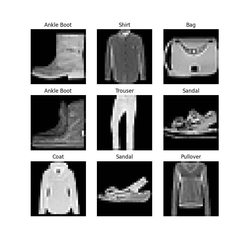
迭代和可视化数据集

我们可以像列表一样手动索引Datasets：training_data[index]。我们使用matplotlib来可视化我们训练数据中的一些样本。

labels_map = {
    0: "T-Shirt",
    1: "Trouser",
    2: "Pullover",
    3: "Dress",
    4: "Coat",
    5: "Sandal",
    6: "Shirt",
    7: "Sneaker",
    8: "Bag",
    9: "Ankle Boot",
}
figure = plt.figure(figsize=(8, 8))
cols, rows = 3, 3
for i in range(1, cols * rows + 1):
    sample_idx = torch.randint(len(training_data), size=(1,)).item()
    img, label = training_data[sample_idx]
    figure.add_subplot(rows, cols, i)
    plt.title(labels_map[label])
    plt.axis("off")
    plt.imshow(img.squeeze(), cmap="gray")
plt.show()

踝靴、衬衫、包、踝靴、裤子、凉鞋、外套、凉鞋、套头衫

为您的文件创建自定义数据集

自定义数据集类必须实现三个函数：__init__、__len__和__getitem__。看一下这个实现；FashionMNIST 图像存储在一个名为img_dir的目录中，它们的标签单独存储在一个名为annotations_file的 CSV 文件中。

在接下来的部分中，我们将分解每个函数中发生的情况。

import os
import pandas as pd
from torchvision.io import read_image

class CustomImageDataset(Dataset):
    def __init__(self, annotations_file, img_dir, transform=None, target_transform=None):
        self.img_labels = pd.read_csv(annotations_file)
        self.img_dir = img_dir
        self.transform = transform
        self.target_transform = target_transform

    def __len__(self):
        return len(self.img_labels)

    def __getitem__(self, idx):
        img_path = os.path.join(self.img_dir, self.img_labels.iloc[idx, 0])
        image = read_image(img_path)
        label = self.img_labels.iloc[idx, 1]
        if self.transform:
            image = self.transform(image)
        if self.target_transform:
            label = self.target_transform(label)
        return image, label

`init`

__init__函数在实例化数据集对象时运行一次。我们初始化包含图像的目录、注释文件和两个转换（在下一节中详细介绍）。

标签.csv 文件如下：

tshirt1.jpg, 0
tshirt2.jpg, 0
......
ankleboot999.jpg, 9

def __init__(self, annotations_file, img_dir, transform=None, target_transform=None):
    self.img_labels = pd.read_csv(annotations_file)
    self.img_dir = img_dir
    self.transform = transform
    self.target_transform = target_transform

`len`

__len__函数返回数据集中样本的数量。

示例：

def __len__(self):
    return len(self.img_labels)

`getitem`

__getitem__函数加载并返回给定索引idx处数据集中的样本。根据索引，它确定磁盘上图像的位置，使用read_image将其转换为张量，从self.img_labels中的 csv 数据中检索相应的标签，对它们调用转换函数（如果适用），并以元组形式返回张量图像和相应标签。

def __getitem__(self, idx):
    img_path = os.path.join(self.img_dir, self.img_labels.iloc[idx, 0])
    image = read_image(img_path)
    label = self.img_labels.iloc[idx, 1]
    if self.transform:
        image = self.transform(image)
    if self.target_transform:
        label = self.target_transform(label)
    return image, label

为使用 DataLoaders 准备数据

Dataset以一次一个样本的方式检索我们数据集的特征和标签。在训练模型时，我们通常希望以“小批量”方式传递样本，每个时代重新洗牌数据以减少模型过拟合，并使用 Python 的multiprocessing加速数据检索。

DataLoader是一个可迭代对象，它在易用的 API 中为我们抽象了这种复杂性。

from torch.utils.data import DataLoader

train_dataloader = DataLoader(training_data, batch_size=64, shuffle=True)
test_dataloader = DataLoader(test_data, batch_size=64, shuffle=True)

遍历 DataLoader

我们已经将数据集加载到DataLoader中，并可以根据需要遍历数据集。下面的每次迭代都会返回一批train_features和train_labels（分别包含batch_size=64个特征和标签）。因为我们指定了shuffle=True，在遍历所有批次后，数据会被洗牌（为了更精细地控制数据加载顺序，请查看Samplers）。

# Display image and label.
train_features, train_labels = next(iter(train_dataloader))
print(f"Feature batch shape: {train_features.size()}")
print(f"Labels batch shape: {train_labels.size()}")
img = train_features[0].squeeze()
label = train_labels[0]
plt.imshow(img, cmap="gray")
plt.show()
print(f"Label: {label}")

数据教程

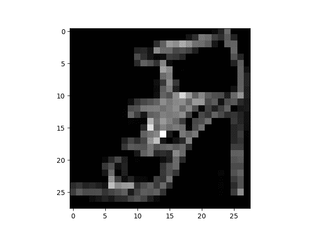
Feature batch shape: torch.Size([64, 1, 28, 28])
Labels batch shape: torch.Size([64])
Label: 5

进一步阅读

torch.utils.data API

脚本的总运行时间：（0 分钟 5.632 秒）

下载 Python 源代码：data_tutorial.py

下载 Jupyter 笔记本：data_tutorial.ipynb

Sphinx-Gallery 生成的画廊

转换

原文：pytorch.org/tutorials/beginner/basics/transforms_tutorial.html

译者：飞龙

协议：CC BY-NC-SA 4.0

注意

点击这里下载完整示例代码

学习基础知识 || 快速入门 || 张量 || 数据集和数据加载器 || 转换 || 构建模型 || 自动求导 || 优化 || 保存和加载模型

数据并不总是以训练机器学习算法所需的最终处理形式出现。我们使用转换对数据进行一些处理，使其适合训练。

所有 TorchVision 数据集都有两个参数-transform用于修改特征和target_transform用于修改标签-接受包含转换逻辑的可调用对象。torchvision.transforms模块提供了几种常用的转换。

FashionMNIST 的特征以 PIL 图像格式呈现，标签为整数。对于训练，我们需要将特征作为标准化张量，将标签作为独热编码张量。为了进行这些转换，我们使用ToTensor和Lambda。

import torch
from torchvision import datasets
from torchvision.transforms import ToTensor, Lambda

ds = datasets.FashionMNIST(
    root="data",
    train=True,
    download=True,
    transform=ToTensor(),
    target_transform=Lambda(lambda y: torch.zeros(10, dtype=torch.float).scatter_(0, torch.tensor(y), value=1))
)

Downloading http://fashion-mnist.s3-website.eu-central-1.amazonaws.com/train-images-idx3-ubyte.gz
Downloading http://fashion-mnist.s3-website.eu-central-1.amazonaws.com/train-images-idx3-ubyte.gz to data/FashionMNIST/raw/train-images-idx3-ubyte.gz

  0%|          | 0/26421880 [00:00<?, ?it/s]
  0%|          | 65536/26421880 [00:00<01:12, 365341.60it/s]
  1%|          | 229376/26421880 [00:00<00:38, 686586.92it/s]
  3%|3         | 884736/26421880 [00:00<00:12, 2035271.39it/s]
 10%|#         | 2686976/26421880 [00:00<00:03, 6286060.82it/s]
 21%|##1       | 5603328/26421880 [00:00<00:01, 10565098.33it/s]
 36%|###5      | 9404416/26421880 [00:00<00:00, 17370347.01it/s]
 54%|#####4    | 14319616/26421880 [00:01<00:00, 21721945.28it/s]
 70%|######9   | 18382848/26421880 [00:01<00:00, 26260208.56it/s]
 90%|########9 | 23724032/26421880 [00:01<00:00, 28093598.52it/s]
100%|##########| 26421880/26421880 [00:01<00:00, 19334744.02it/s]
Extracting data/FashionMNIST/raw/train-images-idx3-ubyte.gz to data/FashionMNIST/raw

Downloading http://fashion-mnist.s3-website.eu-central-1.amazonaws.com/train-labels-idx1-ubyte.gz
Downloading http://fashion-mnist.s3-website.eu-central-1.amazonaws.com/train-labels-idx1-ubyte.gz to data/FashionMNIST/raw/train-labels-idx1-ubyte.gz

  0%|          | 0/29515 [00:00<?, ?it/s]
100%|##########| 29515/29515 [00:00<00:00, 329165.55it/s]
Extracting data/FashionMNIST/raw/train-labels-idx1-ubyte.gz to data/FashionMNIST/raw

Downloading http://fashion-mnist.s3-website.eu-central-1.amazonaws.com/t10k-images-idx3-ubyte.gz
Downloading http://fashion-mnist.s3-website.eu-central-1.amazonaws.com/t10k-images-idx3-ubyte.gz to data/FashionMNIST/raw/t10k-images-idx3-ubyte.gz

  0%|          | 0/4422102 [00:00<?, ?it/s]
  1%|1         | 65536/4422102 [00:00<00:12, 361576.31it/s]
  5%|5         | 229376/4422102 [00:00<00:06, 680517.35it/s]
 21%|##1       | 950272/4422102 [00:00<00:01, 2183882.82it/s]
 77%|#######7  | 3407872/4422102 [00:00<00:00, 6666873.55it/s]
100%|##########| 4422102/4422102 [00:00<00:00, 6066091.89it/s]
Extracting data/FashionMNIST/raw/t10k-images-idx3-ubyte.gz to data/FashionMNIST/raw

Downloading http://fashion-mnist.s3-website.eu-central-1.amazonaws.com/t10k-labels-idx1-ubyte.gz
Downloading http://fashion-mnist.s3-website.eu-central-1.amazonaws.com/t10k-labels-idx1-ubyte.gz to data/FashionMNIST/raw/t10k-labels-idx1-ubyte.gz

  0%|          | 0/5148 [00:00<?, ?it/s]
100%|##########| 5148/5148 [00:00<00:00, 41523609.60it/s]
Extracting data/FashionMNIST/raw/t10k-labels-idx1-ubyte.gz to data/FashionMNIST/raw

ToTensor()

ToTensor将 PIL 图像或 NumPy ndarray转换为FloatTensor。并将图像的像素强度值缩放到范围[0., 1.]内。

Lambda 转换

Lambda 转换应用任何用户定义的 lambda 函数。在这里，我们定义一个函数将整数转换为一个独热编码的张量。它首先创建一个大小为 10 的零张量（数据集中标签的数量），然后调用scatter_，该函数根据标签y给定的索引分配value=1。

target_transform = Lambda(lambda y: torch.zeros(
    10, dtype=torch.float).scatter_(dim=0, index=torch.tensor(y), value=1))

进一步阅读

torchvision.transforms API

脚本的总运行时间：（0 分钟 4.410 秒）

下载 Python 源代码：transforms_tutorial.py

下载 Jupyter 笔记本：transforms_tutorial.ipynb

Sphinx-Gallery 生成的画廊

构建神经网络

原文：pytorch.org/tutorials/beginner/basics/buildmodel_tutorial.html

译者：飞龙

协议：CC BY-NC-SA 4.0

注意

点击这里下载完整示例代码

学习基础知识 || 快速入门 || 张量 || 数据集和数据加载器 || 变换 || 构建模型 || 自动求导 || 优化 || 保存和加载模型

神经网络由在数据上执行操作的层/模块组成。torch.nn 命名空间提供了构建自己的神经网络所需的所有构建模块。PyTorch 中的每个模块都是 nn.Module 的子类。神经网络本身是一个模块，包含其他模块（层）。这种嵌套结构使得轻松构建和管理复杂的架构成为可能。

在接下来的部分中，我们将构建一个神经网络来对 FashionMNIST 数据集中的图像进行分类。

import os
import torch
from torch import nn
from torch.utils.data import DataLoader
from torchvision import datasets, transforms

获取训练设备

如果有可能，我们希望能够在 GPU 或 MPS 等硬件加速器上训练模型。让我们检查一下是否有 torch.cuda 或 torch.backends.mps，否则我们使用 CPU。

device = (
    "cuda"
    if torch.cuda.is_available()
    else "mps"
    if torch.backends.mps.is_available()
    else "cpu"
)
print(f"Using {device} device")

Using cuda device

定义类别

我们通过子类化 nn.Module 来定义我们的神经网络，并在 __init__ 中初始化神经网络层。每个 nn.Module 子类在 forward 方法中实现对输入数据的操作。

class NeuralNetwork(nn.Module):
    def __init__(self):
        super().__init__()
        self.flatten = nn.Flatten()
        self.linear_relu_stack = nn.Sequential(
            nn.Linear(28*28, 512),
            nn.ReLU(),
            nn.Linear(512, 512),
            nn.ReLU(),
            nn.Linear(512, 10),
        )

    def forward(self, x):
        x = self.flatten(x)
        logits = self.linear_relu_stack(x)
        return logits

我们创建一个 NeuralNetwork 实例，并将其移动到 device，然后打印其结构。

model = NeuralNetwork().to(device)
print(model)

NeuralNetwork(
  (flatten): Flatten(start_dim=1, end_dim=-1)
  (linear_relu_stack): Sequential(
    (0): Linear(in_features=784, out_features=512, bias=True)
    (1): ReLU()
    (2): Linear(in_features=512, out_features=512, bias=True)
    (3): ReLU()
    (4): Linear(in_features=512, out_features=10, bias=True)
  )
)

要使用模型，我们将输入数据传递给它。这会执行模型的 forward，以及一些后台操作。不要直接调用 model.forward()！

对输入调用模型会返回一个二维张量，dim=0 对应每个类别的 10 个原始预测值，dim=1 对应每个输出的单个值。通过将其传递给 nn.Softmax 模块，我们可以得到预测概率。

X = torch.rand(1, 28, 28, device=device)
logits = model(X)
pred_probab = nn.Softmax(dim=1)(logits)
y_pred = pred_probab.argmax(1)
print(f"Predicted class: {y_pred}")

Predicted class: tensor([7], device='cuda:0')

模型层

让我们分解 FashionMNIST 模型中的层。为了说明，我们将取一个大小为 28x28 的 3 张图像的示例小批量，并看看当我们将其通过网络时会发生什么。

input_image = torch.rand(3,28,28)
print(input_image.size())

torch.Size([3, 28, 28])

nn.Flatten

我们初始化 nn.Flatten 层，将每个 2D 的 28x28 图像转换为一个连续的包含 784 个像素值的数组（保持 minibatch 维度（在 dim=0））。

flatten = nn.Flatten()
flat_image = flatten(input_image)
print(flat_image.size())

torch.Size([3, 784])

nn.Linear

线性层是一个模块，使用其存储的权重和偏置对输入进行线性变换。

layer1 = nn.Linear(in_features=28*28, out_features=20)
hidden1 = layer1(flat_image)
print(hidden1.size())

torch.Size([3, 20])

nn.ReLU

非线性激活是创建模型输入和输出之间复杂映射的关键。它们在线性变换之后应用，引入 非线性，帮助神经网络学习各种现象。

在这个模型中，我们在线性层之间使用 nn.ReLU，但还有其他激活函数可以引入模型的非线性。

print(f"Before ReLU: {hidden1}\n\n")
hidden1 = nn.ReLU()(hidden1)
print(f"After ReLU: {hidden1}")

Before ReLU: tensor([[ 0.4158, -0.0130, -0.1144,  0.3960,  0.1476, -0.0690, -0.0269,  0.2690,
          0.1353,  0.1975,  0.4484,  0.0753,  0.4455,  0.5321, -0.1692,  0.4504,
          0.2476, -0.1787, -0.2754,  0.2462],
        [ 0.2326,  0.0623, -0.2984,  0.2878,  0.2767, -0.5434, -0.5051,  0.4339,
          0.0302,  0.1634,  0.5649, -0.0055,  0.2025,  0.4473, -0.2333,  0.6611,
          0.1883, -0.1250,  0.0820,  0.2778],
        [ 0.3325,  0.2654,  0.1091,  0.0651,  0.3425, -0.3880, -0.0152,  0.2298,
          0.3872,  0.0342,  0.8503,  0.0937,  0.1796,  0.5007, -0.1897,  0.4030,
          0.1189, -0.3237,  0.2048,  0.4343]], grad_fn=<AddmmBackward0>)

After ReLU: tensor([[0.4158, 0.0000, 0.0000, 0.3960, 0.1476, 0.0000, 0.0000, 0.2690, 0.1353,
         0.1975, 0.4484, 0.0753, 0.4455, 0.5321, 0.0000, 0.4504, 0.2476, 0.0000,
         0.0000, 0.2462],
        [0.2326, 0.0623, 0.0000, 0.2878, 0.2767, 0.0000, 0.0000, 0.4339, 0.0302,
         0.1634, 0.5649, 0.0000, 0.2025, 0.4473, 0.0000, 0.6611, 0.1883, 0.0000,
         0.0820, 0.2778],
        [0.3325, 0.2654, 0.1091, 0.0651, 0.3425, 0.0000, 0.0000, 0.2298, 0.3872,
         0.0342, 0.8503, 0.0937, 0.1796, 0.5007, 0.0000, 0.4030, 0.1189, 0.0000,
         0.2048, 0.4343]], grad_fn=<ReluBackward0>)

nn.Sequential

nn.Sequential 是一个有序的模块容器。数据按照定义的顺序通过所有模块。您可以使用序列容器来组合一个快速网络，比如 seq_modules。

seq_modules = nn.Sequential(
    flatten,
    layer1,
    nn.ReLU(),
    nn.Linear(20, 10)
)
input_image = torch.rand(3,28,28)
logits = seq_modules(input_image)

nn.Softmax

神经网络的最后一个线性层返回 logits - 在[-infty, infty]范围内的原始值 - 这些值传递给nn.Softmax模块。logits 被缩放到表示模型对每个类别的预测概率的值[0, 1]。dim参数指示值必须在其上求和为 1 的维度。

softmax = nn.Softmax(dim=1)
pred_probab = softmax(logits)

模型参数

神经网络内部的许多层都是参数化的，即具有在训练期间优化的相关权重和偏差。通过对nn.Module进行子类化，自动跟踪模型对象内定义的所有字段，并使用模型的parameters()或named_parameters()方法使所有参数可访问。

在这个例子中，我们遍历每个参数，并打印其大小和值的预览。

print(f"Model structure: {model}\n\n")

for name, param in model.named_parameters():
    print(f"Layer: {name} | Size: {param.size()} | Values : {param[:2]}  \n")

Model structure: NeuralNetwork(
  (flatten): Flatten(start_dim=1, end_dim=-1)
  (linear_relu_stack): Sequential(
    (0): Linear(in_features=784, out_features=512, bias=True)
    (1): ReLU()
    (2): Linear(in_features=512, out_features=512, bias=True)
    (3): ReLU()
    (4): Linear(in_features=512, out_features=10, bias=True)
  )
)

Layer: linear_relu_stack.0.weight | Size: torch.Size([512, 784]) | Values : tensor([[ 0.0273,  0.0296, -0.0084,  ..., -0.0142,  0.0093,  0.0135],
        [-0.0188, -0.0354,  0.0187,  ..., -0.0106, -0.0001,  0.0115]],
       device='cuda:0', grad_fn=<SliceBackward0>)

Layer: linear_relu_stack.0.bias | Size: torch.Size([512]) | Values : tensor([-0.0155, -0.0327], device='cuda:0', grad_fn=<SliceBackward0>)

Layer: linear_relu_stack.2.weight | Size: torch.Size([512, 512]) | Values : tensor([[ 0.0116,  0.0293, -0.0280,  ...,  0.0334, -0.0078,  0.0298],
        [ 0.0095,  0.0038,  0.0009,  ..., -0.0365, -0.0011, -0.0221]],
       device='cuda:0', grad_fn=<SliceBackward0>)

Layer: linear_relu_stack.2.bias | Size: torch.Size([512]) | Values : tensor([ 0.0148, -0.0256], device='cuda:0', grad_fn=<SliceBackward0>)

Layer: linear_relu_stack.4.weight | Size: torch.Size([10, 512]) | Values : tensor([[-0.0147, -0.0229,  0.0180,  ..., -0.0013,  0.0177,  0.0070],
        [-0.0202, -0.0417, -0.0279,  ..., -0.0441,  0.0185, -0.0268]],
       device='cuda:0', grad_fn=<SliceBackward0>)

Layer: linear_relu_stack.4.bias | Size: torch.Size([10]) | Values : tensor([ 0.0070, -0.0411], device='cuda:0', grad_fn=<SliceBackward0>)

进一步阅读

torch.nn API

脚本的总运行时间：（0 分钟 2.486 秒）

下载 Python 源代码：buildmodel_tutorial.py

下载 Jupyter 笔记本：buildmodel_tutorial.ipynb

Sphinx-Gallery 生成的图库

使用 torch.autograd 进行自动微分

原文：pytorch.org/tutorials/beginner/basics/autogradqs_tutorial.html

译者：飞龙

协议：CC BY-NC-SA 4.0

注意

点击这里下载完整的示例代码

学习基础知识 || 快速入门 || 张量 || 数据集和数据加载器 || 变换 || 构建模型 || 自动微分 || 优化 || 保存和加载模型

在训练神经网络时，最常用的算法是反向传播。在这个算法中，参数（模型权重）根据损失函数相对于给定参数的梯度进行调整。

为了计算这些梯度，PyTorch 有一个名为torch.autograd的内置微分引擎。它支持对任何计算图进行梯度的自动计算。

考虑最简单的单层神经网络，具有输入x、参数w和b，以及一些损失函数。可以在 PyTorch 中以以下方式定义它：

import torch

x = torch.ones(5)  # input tensor
y = torch.zeros(3)  # expected output
w = torch.randn(5, 3, requires_grad=True)
b = torch.randn(3, requires_grad=True)
z = torch.matmul(x, w)+b
loss = torch.nn.functional.binary_cross_entropy_with_logits(z, y)

张量、函数和计算图

这段代码定义了以下计算图：

在这个网络中，w和b是参数，我们需要优化它们。因此，我们需要能够计算损失函数相对于这些变量的梯度。为了做到这一点，我们设置这些张量的requires_grad属性。

注意

您可以在创建张量时设置requires_grad的值，或稍后使用x.requires_grad_(True)方法设置。

我们应用于张量以构建计算图的函数实际上是Function类的对象。这个对象知道如何在前向方向计算函数，也知道如何在反向传播步骤中计算它的导数。反向传播函数的引用存储在张量的grad_fn属性中。您可以在文档中找到有关Function的更多信息。

print(f"Gradient function for z = {z.grad_fn}")
print(f"Gradient function for loss = {loss.grad_fn}")

Gradient function for z = <AddBackward0 object at 0x7f1bd884c130>
Gradient function for loss = <BinaryCrossEntropyWithLogitsBackward0 object at 0x7f1bd884c670>

计算梯度

为了优化神经网络中参数的权重，我们需要计算损失函数相对于参数的导数，即我们需要在一些固定的x和y值下计算 $\frac{\partial loss}{\partial w}$ 和 $\frac{\partial loss}{\partial b}$ 。要计算这些导数，我们调用loss.backward()，然后从w.grad和b.grad中检索值：

loss.backward()
print(w.grad)
print(b.grad)

tensor([[0.3313, 0.0626, 0.2530],
        [0.3313, 0.0626, 0.2530],
        [0.3313, 0.0626, 0.2530],
        [0.3313, 0.0626, 0.2530],
        [0.3313, 0.0626, 0.2530]])
tensor([0.3313, 0.0626, 0.2530])

注意

我们只能获取计算图的叶节点的grad属性，这些叶节点的requires_grad属性设置为True。对于图中的所有其他节点，梯度将不可用。
出于性能原因，我们只能在给定图上一次使用backward进行梯度计算。如果我们需要在同一图上进行多次backward调用，我们需要在backward调用中传递retain_graph=True。

禁用梯度跟踪

默认情况下，所有requires_grad=True的张量都在跟踪它们的计算历史并支持梯度计算。然而，在某些情况下，我们不需要这样做，例如，当我们已经训练好模型，只想将其应用于一些输入数据时，即我们只想通过网络进行前向计算。我们可以通过在计算代码周围加上torch.no_grad()块来停止跟踪计算：

z = torch.matmul(x, w)+b
print(z.requires_grad)

with torch.no_grad():
    z = torch.matmul(x, w)+b
print(z.requires_grad)

True
False

实现相同结果的另一种方法是在张量上使用detach()方法：

z = torch.matmul(x, w)+b
z_det = z.detach()
print(z_det.requires_grad)

False

有一些原因您可能希望禁用梯度跟踪：

将神经网络中的一些参数标记为冻结参数。
在只进行前向传递时加速计算，因为不跟踪梯度的张量上的计算会更有效率。

关于计算图的更多信息

从概念上讲，autograd 在有向无环图（DAG）中保留了数据（张量）和所有执行的操作（以及生成的新张量）的记录，这些操作由Function对象组成。在这个 DAG 中，叶子是输入张量，根是输出张量。通过从根到叶子追踪这个图，您可以使用链式法则自动计算梯度。

在前向传递中，autograd 同时执行两个操作：

运行请求的操作以计算生成的张量
在 DAG 中维护操作的梯度函数。

当在 DAG 根上调用.backward()时，反向传递开始。然后autograd：

计算每个.grad_fn的梯度，
在相应张量的.grad属性中累积它们
使用链式法则，将所有内容传播到叶张量。

注意

PyTorch 中的 DAGs 是动态的 需要注意的一点是，图是从头开始重新创建的；在每次.backward()调用之后，autograd 开始填充一个新图。这正是允许您在模型中使用控制流语句的原因；如果需要，您可以在每次迭代中更改形状、大小和操作。

可选阅读：张量梯度和 Jacobian 乘积

在许多情况下，我们有一个标量损失函数，需要计算相对于某些参数的梯度。然而，有些情况下输出函数是任意张量。在这种情况下，PyTorch 允许您计算所谓的Jacobian product，而不是实际梯度。

对于向量函数 $\vec{y}=f(\vec{x})$ ，其中 $\vec{x}=\langle x_1,\dots,x_n\rangle$ 和 $\vec{y}=\langle y_1,\dots,y_m\rangle$ ， $\vec{y}$ 相对于 $\vec{x}$ 的梯度由Jacobian 矩阵给出：

$J=\left(\begin{array}{ccc} \frac{\partial y_{1}}{\partial x_{1}} & \cdots & \frac{\partial y_{1}}{\partial x_{n}}\\ \vdots & \ddots & \vdots\\ \frac{\partial y_{m}}{\partial x_{1}} & \cdots & \frac{\partial y_{m}}{\partial x_{n}} \end{array}\right)$

PyTorch 允许您计算给定输入向量 $v=(v_1 \dots v_m)$ 的Jacobian Product $v^T\cdot J$ ，而不是计算 Jacobian 矩阵本身。通过使用 $v$ 作为参数调用backward来实现这一点。 $v$ 的大小应该与原始张量的大小相同，我们希望计算乘积的大小：

inp = torch.eye(4, 5, requires_grad=True)
out = (inp+1).pow(2).t()
out.backward(torch.ones_like(out), retain_graph=True)
print(f"First call\n{inp.grad}")
out.backward(torch.ones_like(out), retain_graph=True)
print(f"\nSecond call\n{inp.grad}")
inp.grad.zero_()
out.backward(torch.ones_like(out), retain_graph=True)
print(f"\nCall after zeroing gradients\n{inp.grad}")

First call
tensor([[4., 2., 2., 2., 2.],
        [2., 4., 2., 2., 2.],
        [2., 2., 4., 2., 2.],
        [2., 2., 2., 4., 2.]])

Second call
tensor([[8., 4., 4., 4., 4.],
        [4., 8., 4., 4., 4.],
        [4., 4., 8., 4., 4.],
        [4., 4., 4., 8., 4.]])

Call after zeroing gradients
tensor([[4., 2., 2., 2., 2.],
        [2., 4., 2., 2., 2.],
        [2., 2., 4., 2., 2.],
        [2., 2., 2., 4., 2.]])

请注意，当我们第二次使用相同参数调用backward时，梯度的值是不同的。这是因为在进行backward传播时，PyTorch 累积梯度，即计算出的梯度值被添加到计算图的所有叶节点的grad属性中。如果要计算正确的梯度，需要在之前将grad属性清零。在实际训练中，优化器帮助我们做到这一点。

注意

以前我们在没有参数的情况下调用backward()函数。这本质上等同于调用backward(torch.tensor(1.0))，这是在神经网络训练中计算标量值函数（如损失）梯度的一种有用方式。

进一步阅读

Autograd Mechanics

脚本的总运行时间：（0 分钟 1.594 秒）

下载 Python 源代码：autogradqs_tutorial.py

下载 Jupyter 笔记本：autogradqs_tutorial.ipynb

Sphinx-Gallery 生成的画廊

优化模型参数

原文：pytorch.org/tutorials/beginner/basics/optimization_tutorial.html

译者：飞龙

协议：CC BY-NC-SA 4.0

注意

点击这里下载完整示例代码

学习基础知识 || 快速入门 || 张量 || 数据集和数据加载器 || 转换 || 构建模型 || 自动求导 || 优化 || 保存和加载模型

现在我们有了模型和数据，是时候通过优化其参数在数据上训练、验证和测试我们的模型了。训练模型是一个迭代过程；在每次迭代中，模型对输出进行猜测，计算其猜测的错误（损失），收集关于其参数的错误的导数（正如我们在上一节中看到的），并使用梯度下降优化这些参数。要了解此过程的更详细步骤，请查看这个关于3Blue1Brown 的反向传播视频。

先决条件代码

我们加载了前几节关于数据集和数据加载器和构建模型的代码。

import torch
from torch import nn
from torch.utils.data import DataLoader
from torchvision import datasets
from torchvision.transforms import ToTensor

training_data = datasets.FashionMNIST(
    root="data",
    train=True,
    download=True,
    transform=ToTensor()
)

test_data = datasets.FashionMNIST(
    root="data",
    train=False,
    download=True,
    transform=ToTensor()
)

train_dataloader = DataLoader(training_data, batch_size=64)
test_dataloader = DataLoader(test_data, batch_size=64)

class NeuralNetwork(nn.Module):
    def __init__(self):
        super().__init__()
        self.flatten = nn.Flatten()
        self.linear_relu_stack = nn.Sequential(
            nn.Linear(28*28, 512),
            nn.ReLU(),
            nn.Linear(512, 512),
            nn.ReLU(),
            nn.Linear(512, 10),
        )

    def forward(self, x):
        x = self.flatten(x)
        logits = self.linear_relu_stack(x)
        return logits

model = NeuralNetwork()

Downloading http://fashion-mnist.s3-website.eu-central-1.amazonaws.com/train-images-idx3-ubyte.gz
Downloading http://fashion-mnist.s3-website.eu-central-1.amazonaws.com/train-images-idx3-ubyte.gz to data/FashionMNIST/raw/train-images-idx3-ubyte.gz

  0%|          | 0/26421880 [00:00<?, ?it/s]
  0%|          | 65536/26421880 [00:00<01:12, 365539.83it/s]
  1%|          | 229376/26421880 [00:00<00:38, 684511.48it/s]
  3%|3         | 884736/26421880 [00:00<00:12, 2030637.83it/s]
 12%|#1        | 3080192/26421880 [00:00<00:03, 6027159.86it/s]
 31%|###       | 8060928/26421880 [00:00<00:01, 16445259.09it/s]
 42%|####1     | 11075584/26421880 [00:00<00:00, 16871356.21it/s]
 64%|######3   | 16908288/26421880 [00:01<00:00, 24452744.90it/s]
 76%|#######6  | 20086784/26421880 [00:01<00:00, 24276135.68it/s]
 98%|#########7| 25788416/26421880 [00:01<00:00, 32055536.22it/s]
100%|##########| 26421880/26421880 [00:01<00:00, 18270891.31it/s]
Extracting data/FashionMNIST/raw/train-images-idx3-ubyte.gz to data/FashionMNIST/raw

Downloading http://fashion-mnist.s3-website.eu-central-1.amazonaws.com/train-labels-idx1-ubyte.gz
Downloading http://fashion-mnist.s3-website.eu-central-1.amazonaws.com/train-labels-idx1-ubyte.gz to data/FashionMNIST/raw/train-labels-idx1-ubyte.gz

  0%|          | 0/29515 [00:00<?, ?it/s]
100%|##########| 29515/29515 [00:00<00:00, 326183.74it/s]
Extracting data/FashionMNIST/raw/train-labels-idx1-ubyte.gz to data/FashionMNIST/raw

Downloading http://fashion-mnist.s3-website.eu-central-1.amazonaws.com/t10k-images-idx3-ubyte.gz
Downloading http://fashion-mnist.s3-website.eu-central-1.amazonaws.com/t10k-images-idx3-ubyte.gz to data/FashionMNIST/raw/t10k-images-idx3-ubyte.gz

  0%|          | 0/4422102 [00:00<?, ?it/s]
  1%|1         | 65536/4422102 [00:00<00:12, 361771.90it/s]
  5%|5         | 229376/4422102 [00:00<00:06, 680798.45it/s]
 21%|##        | 917504/4422102 [00:00<00:01, 2100976.96it/s]
 70%|#######   | 3112960/4422102 [00:00<00:00, 6040440.05it/s]
100%|##########| 4422102/4422102 [00:00<00:00, 6047736.61it/s]
Extracting data/FashionMNIST/raw/t10k-images-idx3-ubyte.gz to data/FashionMNIST/raw

Downloading http://fashion-mnist.s3-website.eu-central-1.amazonaws.com/t10k-labels-idx1-ubyte.gz
Downloading http://fashion-mnist.s3-website.eu-central-1.amazonaws.com/t10k-labels-idx1-ubyte.gz to data/FashionMNIST/raw/t10k-labels-idx1-ubyte.gz

  0%|          | 0/5148 [00:00<?, ?it/s]
100%|##########| 5148/5148 [00:00<00:00, 36846889.06it/s]
Extracting data/FashionMNIST/raw/t10k-labels-idx1-ubyte.gz to data/FashionMNIST/raw

超参数

超参数是可调参数，让您控制模型优化过程。不同的超参数值可能会影响模型训练和收敛速度（了解更多关于超参数调整）

我们为训练定义以下超参数：

Epoch 的数量 - 数据集迭代的次数
批量大小 - 在更新参数之前通过网络传播的数据样本数量
学习率 - 每个批次/epoch 更新模型参数的量。较小的值会导致学习速度较慢，而较大的值可能会导致训练过程中出现不可预测的行为。

learning_rate = 1e-3
batch_size = 64
epochs = 5

优化循环

一旦设置了超参数，我们就可以通过优化循环训练和优化我们的模型。优化循环的每次迭代称为epoch。

每个 epoch 包括两个主要部分：

训练循环 - 迭代训练数据集并尝试收敛到最佳参数。
验证/测试循环 - 迭代测试数据集以检查模型性能是否改善。

让我们简要了解一下训练循环中使用的一些概念。跳转到完整实现以查看优化循环。

损失函数

当给定一些训练数据时，我们未经训练的网络可能不会给出正确答案。损失函数衡量获得的结果与目标值的不相似程度，我们希望在训练过程中最小化损失函数。为了计算损失，我们使用给定数据样本的输入进行预测，并将其与真实数据标签值进行比较。

常见的损失函数包括nn.MSELoss（均方误差）用于回归任务，以及nn.NLLLoss（负对数似然）用于分类。nn.CrossEntropyLoss结合了nn.LogSoftmax和nn.NLLLoss。

我们将模型的输出 logits 传递给nn.CrossEntropyLoss，它将对 logits 进行归一化并计算预测错误。

# Initialize the loss function
loss_fn = nn.CrossEntropyLoss()

优化器

优化是调整模型参数以减少每个训练步骤中模型误差的过程。优化算法定义了如何执行这个过程（在这个例子中我们使用随机梯度下降）。所有的优化逻辑都封装在optimizer对象中。在这里，我们使用 SGD 优化器；此外，PyTorch 还有许多不同的优化器可供选择，如 ADAM 和 RMSProp，适用于不同类型的模型和数据。

我们通过注册需要训练的模型参数并传入学习率超参数来初始化优化器。

optimizer = torch.optim.SGD(model.parameters(), lr=learning_rate)

在训练循环中，优化分为三个步骤：

调用optimizer.zero_grad()来重置模型参数的梯度。梯度默认会累加；为了防止重复计算，我们在每次迭代时明确将其归零。
通过调用loss.backward()来反向传播预测损失。PyTorch 会将损失相对于每个参数的梯度存储起来。
一旦我们有了梯度，我们调用optimizer.step()来根据反向传播中收集的梯度调整参数。

完整实现

我们定义train_loop循环优化代码，并定义test_loop评估模型在测试数据上的性能。

def train_loop(dataloader, model, loss_fn, optimizer):
    size = len(dataloader.dataset)
    # Set the model to training mode - important for batch normalization and dropout layers
    # Unnecessary in this situation but added for best practices
    model.train()
    for batch, (X, y) in enumerate(dataloader):
        # Compute prediction and loss
        pred = model(X)
        loss = loss_fn(pred, y)

        # Backpropagation
        loss.backward()
        optimizer.step()
        optimizer.zero_grad()

        if batch % 100 == 0:
            loss, current = loss.item(), batch * batch_size + len(X)
            print(f"loss: {loss:>7f} [{current:>5d}/{size:>5d}]")

def test_loop(dataloader, model, loss_fn):
    # Set the model to evaluation mode - important for batch normalization and dropout layers
    # Unnecessary in this situation but added for best practices
    model.eval()
    size = len(dataloader.dataset)
    num_batches = len(dataloader)
    test_loss, correct = 0, 0

    # Evaluating the model with torch.no_grad() ensures that no gradients are computed during test mode
    # also serves to reduce unnecessary gradient computations and memory usage for tensors with requires_grad=True
    with torch.no_grad():
        for X, y in dataloader:
            pred = model(X)
            test_loss += loss_fn(pred, y).item()
            correct += (pred.argmax(1) == y).type(torch.float).sum().item()

    test_loss /= num_batches
    correct /= size
    print(f"Test Error: \n Accuracy: {(100*correct):>0.1f}%, Avg loss: {test_loss:>8f}  \n")

我们初始化损失函数和优化器，并将其传递给train_loop和test_loop。可以增加 epoch 的数量来跟踪模型的性能改进。

loss_fn = nn.CrossEntropyLoss()
optimizer = torch.optim.SGD(model.parameters(), lr=learning_rate)

epochs = 10
for t in range(epochs):
    print(f"Epoch {t+1}\n-------------------------------")
    train_loop(train_dataloader, model, loss_fn, optimizer)
    test_loop(test_dataloader, model, loss_fn)
print("Done!")

Epoch 1
-------------------------------
loss: 2.298730  [   64/60000]
loss: 2.289123  [ 6464/60000]
loss: 2.273286  [12864/60000]
loss: 2.269406  [19264/60000]
loss: 2.249603  [25664/60000]
loss: 2.229407  [32064/60000]
loss: 2.227368  [38464/60000]
loss: 2.204261  [44864/60000]
loss: 2.206193  [51264/60000]
loss: 2.166651  [57664/60000]
Test Error:
 Accuracy: 50.9%, Avg loss: 2.166725

Epoch 2
-------------------------------
loss: 2.176750  [   64/60000]
loss: 2.169595  [ 6464/60000]
loss: 2.117500  [12864/60000]
loss: 2.129272  [19264/60000]
loss: 2.079674  [25664/60000]
loss: 2.032928  [32064/60000]
loss: 2.050115  [38464/60000]
loss: 1.985236  [44864/60000]
loss: 1.987887  [51264/60000]
loss: 1.907162  [57664/60000]
Test Error:
 Accuracy: 55.9%, Avg loss: 1.915486

Epoch 3
-------------------------------
loss: 1.951612  [   64/60000]
loss: 1.928685  [ 6464/60000]
loss: 1.815709  [12864/60000]
loss: 1.841552  [19264/60000]
loss: 1.732467  [25664/60000]
loss: 1.692914  [32064/60000]
loss: 1.701714  [38464/60000]
loss: 1.610632  [44864/60000]
loss: 1.632870  [51264/60000]
loss: 1.514263  [57664/60000]
Test Error:
 Accuracy: 58.8%, Avg loss: 1.541525

Epoch 4
-------------------------------
loss: 1.616448  [   64/60000]
loss: 1.582892  [ 6464/60000]
loss: 1.427595  [12864/60000]
loss: 1.487950  [19264/60000]
loss: 1.359332  [25664/60000]
loss: 1.364817  [32064/60000]
loss: 1.371491  [38464/60000]
loss: 1.298706  [44864/60000]
loss: 1.336201  [51264/60000]
loss: 1.232145  [57664/60000]
Test Error:
 Accuracy: 62.2%, Avg loss: 1.260237

Epoch 5
-------------------------------
loss: 1.345538  [   64/60000]
loss: 1.327798  [ 6464/60000]
loss: 1.153802  [12864/60000]
loss: 1.254829  [19264/60000]
loss: 1.117322  [25664/60000]
loss: 1.153248  [32064/60000]
loss: 1.171765  [38464/60000]
loss: 1.110263  [44864/60000]
loss: 1.154467  [51264/60000]
loss: 1.070921  [57664/60000]
Test Error:
 Accuracy: 64.1%, Avg loss: 1.089831

Epoch 6
-------------------------------
loss: 1.166889  [   64/60000]
loss: 1.170514  [ 6464/60000]
loss: 0.979435  [12864/60000]
loss: 1.113774  [19264/60000]
loss: 0.973411  [25664/60000]
loss: 1.015192  [32064/60000]
loss: 1.051113  [38464/60000]
loss: 0.993591  [44864/60000]
loss: 1.039709  [51264/60000]
loss: 0.971077  [57664/60000]
Test Error:
 Accuracy: 65.8%, Avg loss: 0.982440

Epoch 7
-------------------------------
loss: 1.045165  [   64/60000]
loss: 1.070583  [ 6464/60000]
loss: 0.862304  [12864/60000]
loss: 1.022265  [19264/60000]
loss: 0.885213  [25664/60000]
loss: 0.919528  [32064/60000]
loss: 0.972762  [38464/60000]
loss: 0.918728  [44864/60000]
loss: 0.961629  [51264/60000]
loss: 0.904379  [57664/60000]
Test Error:
 Accuracy: 66.9%, Avg loss: 0.910167

Epoch 8
-------------------------------
loss: 0.956964  [   64/60000]
loss: 1.002171  [ 6464/60000]
loss: 0.779057  [12864/60000]
loss: 0.958409  [19264/60000]
loss: 0.827240  [25664/60000]
loss: 0.850262  [32064/60000]
loss: 0.917320  [38464/60000]
loss: 0.868384  [44864/60000]
loss: 0.905506  [51264/60000]
loss: 0.856353  [57664/60000]
Test Error:
 Accuracy: 68.3%, Avg loss: 0.858248

Epoch 9
-------------------------------
loss: 0.889765  [   64/60000]
loss: 0.951220  [ 6464/60000]
loss: 0.717035  [12864/60000]
loss: 0.911042  [19264/60000]
loss: 0.786085  [25664/60000]
loss: 0.798370  [32064/60000]
loss: 0.874939  [38464/60000]
loss: 0.832796  [44864/60000]
loss: 0.863254  [51264/60000]
loss: 0.819742  [57664/60000]
Test Error:
 Accuracy: 69.5%, Avg loss: 0.818780

Epoch 10
-------------------------------
loss: 0.836395  [   64/60000]
loss: 0.910220  [ 6464/60000]
loss: 0.668506  [12864/60000]
loss: 0.874338  [19264/60000]
loss: 0.754805  [25664/60000]
loss: 0.758453  [32064/60000]
loss: 0.840451  [38464/60000]
loss: 0.806153  [44864/60000]
loss: 0.830360  [51264/60000]
loss: 0.790281  [57664/60000]
Test Error:
 Accuracy: 71.0%, Avg loss: 0.787271

Done!

进一步阅读

损失函数
torch.optim
热启动训练模型

脚本的总运行时间：（2 分钟 0.365 秒）

下载 Python 源代码：optimization_tutorial.py

下载 Jupyter 笔记本：optimization_tutorial.ipynb

Sphinx-Gallery 生成的图库

保存和加载模型

原文：pytorch.org/tutorials/beginner/basics/saveloadrun_tutorial.html

译者：飞龙

协议：CC BY-NC-SA 4.0

注意

点击这里下载完整示例代码

学习基础知识 || 快速入门 || 张量 || 数据集和数据加载器 || 转换 || 构建模型 || 自动求导 || 优化 || 保存和加载模型

在本节中，我们将看看如何通过保存、加载和运行模型预测来持久化模型状态。

import torch
import torchvision.models as models

保存和加载模型权重

PyTorch 模型将学习到的参数存储在内部状态字典中，称为 state_dict。这些可以通过 torch.save 方法进行持久化：

model = models.vgg16(weights='IMAGENET1K_V1')
torch.save(model.state_dict(), 'model_weights.pth')

Downloading: "https://download.pytorch.org/models/vgg16-397923af.pth" to /var/lib/jenkins/.cache/torch/hub/checkpoints/vgg16-397923af.pth

  0%|          | 0.00/528M [00:00<?, ?B/s]
  2%|2         | 12.7M/528M [00:00<00:04, 133MB/s]
  5%|4         | 25.9M/528M [00:00<00:03, 136MB/s]
  8%|7         | 40.3M/528M [00:00<00:03, 143MB/s]
 10%|#         | 54.0M/528M [00:00<00:03, 141MB/s]
 13%|#2        | 67.4M/528M [00:00<00:03, 138MB/s]
 15%|#5        | 81.8M/528M [00:00<00:03, 142MB/s]
 18%|#8        | 96.2M/528M [00:00<00:03, 145MB/s]
 21%|##        | 110M/528M [00:00<00:03, 145MB/s]
 24%|##3       | 124M/528M [00:00<00:02, 147MB/s]
 26%|##6       | 139M/528M [00:01<00:02, 148MB/s]
 29%|##9       | 153M/528M [00:01<00:02, 149MB/s]
 32%|###1      | 168M/528M [00:01<00:02, 150MB/s]
 35%|###4      | 182M/528M [00:01<00:02, 151MB/s]
 37%|###7      | 197M/528M [00:01<00:02, 123MB/s]
 40%|###9      | 210M/528M [00:01<00:02, 127MB/s]
 42%|####2     | 223M/528M [00:01<00:02, 113MB/s]
 44%|####4     | 234M/528M [00:01<00:02, 112MB/s]
 47%|####6     | 248M/528M [00:01<00:02, 119MB/s]
 50%|####9     | 262M/528M [00:02<00:02, 128MB/s]
 52%|#####2    | 275M/528M [00:02<00:02, 129MB/s]
 55%|#####4    | 288M/528M [00:02<00:01, 132MB/s]
 57%|#####7    | 302M/528M [00:02<00:01, 136MB/s]
 60%|#####9    | 316M/528M [00:02<00:01, 140MB/s]
 63%|######2   | 331M/528M [00:02<00:01, 144MB/s]
 65%|######5   | 345M/528M [00:02<00:01, 146MB/s]
 68%|######8   | 360M/528M [00:02<00:01, 148MB/s]
 71%|#######   | 374M/528M [00:02<00:01, 149MB/s]
 74%|#######3  | 389M/528M [00:02<00:00, 150MB/s]
 76%|#######6  | 403M/528M [00:03<00:00, 151MB/s]
 79%|#######9  | 418M/528M [00:03<00:00, 151MB/s]
 82%|########1 | 432M/528M [00:03<00:00, 151MB/s]
 85%|########4 | 447M/528M [00:03<00:00, 152MB/s]
 87%|########7 | 461M/528M [00:03<00:00, 152MB/s]
 90%|######### | 476M/528M [00:03<00:00, 152MB/s]
 93%|#########2| 490M/528M [00:03<00:00, 152MB/s]
 96%|#########5| 505M/528M [00:03<00:00, 151MB/s]
 98%|#########8| 519M/528M [00:03<00:00, 151MB/s]
100%|##########| 528M/528M [00:03<00:00, 142MB/s]

要加载模型权重，您需要首先创建相同模型的实例，然后使用 load_state_dict() 方法加载参数。

model = models.vgg16() # we do not specify ``weights``, i.e. create untrained model
model.load_state_dict(torch.load('model_weights.pth'))
model.eval()

VGG(
  (features): Sequential(
    (0): Conv2d(3, 64, kernel_size=(3, 3), stride=(1, 1), padding=(1, 1))
    (1): ReLU(inplace=True)
    (2): Conv2d(64, 64, kernel_size=(3, 3), stride=(1, 1), padding=(1, 1))
    (3): ReLU(inplace=True)
    (4): MaxPool2d(kernel_size=2, stride=2, padding=0, dilation=1, ceil_mode=False)
    (5): Conv2d(64, 128, kernel_size=(3, 3), stride=(1, 1), padding=(1, 1))
    (6): ReLU(inplace=True)
    (7): Conv2d(128, 128, kernel_size=(3, 3), stride=(1, 1), padding=(1, 1))
    (8): ReLU(inplace=True)
    (9): MaxPool2d(kernel_size=2, stride=2, padding=0, dilation=1, ceil_mode=False)
    (10): Conv2d(128, 256, kernel_size=(3, 3), stride=(1, 1), padding=(1, 1))
    (11): ReLU(inplace=True)
    (12): Conv2d(256, 256, kernel_size=(3, 3), stride=(1, 1), padding=(1, 1))
    (13): ReLU(inplace=True)
    (14): Conv2d(256, 256, kernel_size=(3, 3), stride=(1, 1), padding=(1, 1))
    (15): ReLU(inplace=True)
    (16): MaxPool2d(kernel_size=2, stride=2, padding=0, dilation=1, ceil_mode=False)
    (17): Conv2d(256, 512, kernel_size=(3, 3), stride=(1, 1), padding=(1, 1))
    (18): ReLU(inplace=True)
    (19): Conv2d(512, 512, kernel_size=(3, 3), stride=(1, 1), padding=(1, 1))
    (20): ReLU(inplace=True)
    (21): Conv2d(512, 512, kernel_size=(3, 3), stride=(1, 1), padding=(1, 1))
    (22): ReLU(inplace=True)
    (23): MaxPool2d(kernel_size=2, stride=2, padding=0, dilation=1, ceil_mode=False)
    (24): Conv2d(512, 512, kernel_size=(3, 3), stride=(1, 1), padding=(1, 1))
    (25): ReLU(inplace=True)
    (26): Conv2d(512, 512, kernel_size=(3, 3), stride=(1, 1), padding=(1, 1))
    (27): ReLU(inplace=True)
    (28): Conv2d(512, 512, kernel_size=(3, 3), stride=(1, 1), padding=(1, 1))
    (29): ReLU(inplace=True)
    (30): MaxPool2d(kernel_size=2, stride=2, padding=0, dilation=1, ceil_mode=False)
  )
  (avgpool): AdaptiveAvgPool2d(output_size=(7, 7))
  (classifier): Sequential(
    (0): Linear(in_features=25088, out_features=4096, bias=True)
    (1): ReLU(inplace=True)
    (2): Dropout(p=0.5, inplace=False)
    (3): Linear(in_features=4096, out_features=4096, bias=True)
    (4): ReLU(inplace=True)
    (5): Dropout(p=0.5, inplace=False)
    (6): Linear(in_features=4096, out_features=1000, bias=True)
  )
)