电商分析
1 案例:某年淘宝双12部分购物数据
1.1 数据:某年淘宝双12部分购物数据;
来源:天池数据平台
1.2 分析目的:
- 熟悉电商常用分析指标
- 用户行为分析
- 用户价值模型
2 熟悉数据
2.1 导入数据
import pandas as pd
fpath = r'data\data.csv'
pdata = pd.read_csv(fpath)
pdata.columns
Index(['user_id', 'item_id', 'behavior_type', 'user_geohash', 'item_category',
       'time'],
      dtype='object')
| 字段 | 字段说明 | 提取说明 |
|---|---|---|
| user_id | 用户标识 | 抽样&字段脱敏(非真实ID) |
| item_id | 商品标识 | 字段脱敏(非真实ID) |
| behavior_type | 用户对商品的行为类型 | 包括浏览、收藏、加购物车、购买,对应取值分别是1、2、3、4。 |
| user_geohash | 用户位置的空间标识,可以为空 | 由经纬度通过保密的算法生成 |
| item_category | 商品分类标识 | 字段脱敏 |
| time | 行为时间 | 精确到 a cell. |
pdata
| user_id | item_id | behavior_type | user_geohash | item_category | time | |
|---|---|---|---|---|---|---|
| 0 | 98047837 | 232431562 | 1 | NaN | 4245 | 2014-12-06 02 |
| 1 | 97726136 | 383583590 | 1 | NaN | 5894 | 2014-12-09 20 |
| 2 | 98607707 | 64749712 | 1 | NaN | 2883 | 2014-12-18 11 |
| 3 | 98662432 | 320593836 | 1 | 96nn52n | 6562 | 2014-12-06 10 |
| 4 | 98145908 | 290208520 | 1 | NaN | 13926 | 2014-12-16 21 |
| ... | ... | ... | ... | ... | ... | ... |
| 12256901 | 93812622 | 378365755 | 1 | 95q6d6a | 11 | 2014-12-13 21 |
| 12256902 | 93812622 | 177724753 | 1 | NaN | 12311 | 2014-12-14 21 |
| 12256903 | 93812622 | 234391443 | 1 | NaN | 8765 | 2014-12-11 16 |
| 12256904 | 93812622 | 26452000 | 1 | 95q6dqc | 7951 | 2014-12-08 22 |
| 12256905 | 108404535 | 362699797 | 1 | NaN | 9847 | 2014-12-03 19 |
12256906 rows × 6 columns
# 数据量大小
len(pdata)
12256906
#判断缺失数据计算
missAll = pdata.isnull().sum()
missAll
user_id                0
item_id                0
behavior_type          0
user_geohash     8334824
item_category          0
time                   0
dtype: int64
#统计缺失字段
missField = missAll[missAll>0]
missField
user_geohash    8334824
dtype: int64
2.2 基本分析
指标:PV与UV
- PV(访问量):Page View,览量/点击量(包括重复浏览)。
- UV(独立访客):Unique Visitor, 独立用户或者设备访问量。。
#将字符串时间转成Timestamp
pdata['ts'] = pd.to_datetime(pdata['time'])
pdata['hour'] = pdata.ts.map(lambda item: item.hour)
pdata['day'] =pdata.ts.map(lambda item: item.date())
pdata
| user_id | item_id | behavior_type | user_geohash | item_category | time | ts | hour | day | |
|---|---|---|---|---|---|---|---|---|---|
| 0 | 98047837 | 232431562 | 1 | NaN | 4245 | 2014-12-06 02 | 2014-12-06 02:00:00 | 2 | 2014-12-06 |
| 1 | 97726136 | 383583590 | 1 | NaN | 5894 | 2014-12-09 20 | 2014-12-09 20:00:00 | 20 | 2014-12-09 |
| 2 | 98607707 | 64749712 | 1 | NaN | 2883 | 2014-12-18 11 | 2014-12-18 11:00:00 | 11 | 2014-12-18 |
| 3 | 98662432 | 320593836 | 1 | 96nn52n | 6562 | 2014-12-06 10 | 2014-12-06 10:00:00 | 10 | 2014-12-06 |
| 4 | 98145908 | 290208520 | 1 | NaN | 13926 | 2014-12-16 21 | 2014-12-16 21:00:00 | 21 | 2014-12-16 |
| ... | ... | ... | ... | ... | ... | ... | ... | ... | ... |
| 12256901 | 93812622 | 378365755 | 1 | 95q6d6a | 11 | 2014-12-13 21 | 2014-12-13 21:00:00 | 21 | 2014-12-13 |
| 12256902 | 93812622 | 177724753 | 1 | NaN | 12311 | 2014-12-14 21 | 2014-12-14 21:00:00 | 21 | 2014-12-14 |
| 12256903 | 93812622 | 234391443 | 1 | NaN | 8765 | 2014-12-11 16 | 2014-12-11 16:00:00 | 16 | 2014-12-11 |
| 12256904 | 93812622 | 26452000 | 1 | 95q6dqc | 7951 | 2014-12-08 22 | 2014-12-08 22:00:00 | 22 | 2014-12-08 |
| 12256905 | 108404535 | 362699797 | 1 | NaN | 9847 | 2014-12-03 19 | 2014-12-03 19:00:00 | 19 | 2014-12-03 |
12256906 rows × 9 columns
#PV分析:每天访问量
daily_pv = pdata.groupby('day')['user_id'].count()
daily_pv
day
2014-11-18    366701
2014-11-19    358823
2014-11-20    353429
2014-11-21    333104
2014-11-22    361355
2014-11-23    382702
2014-11-24    378342
2014-11-25    370239
2014-11-26    360896
2014-11-27    371384
2014-11-28    340638
2014-11-29    364697
2014-11-30    401620
2014-12-01    394611
2014-12-02    405216
2014-12-03    411606
2014-12-04    399952
2014-12-05    361878
2014-12-06    389610
2014-12-07    399751
2014-12-08    386667
2014-12-09    398025
2014-12-10    421910
2014-12-11    488508
2014-12-12    691712
2014-12-13    407160
2014-12-14    402541
2014-12-15    398356
2014-12-16    395085
2014-12-17    384791
2014-12-18    375597
Name: user_id, dtype: int64
# UV分析:每天独立用户数
tmp = pdata.groupby('day')['user_id']
#每个分组去重,并统计数量
daily_uv = tmp.apply(lambda x:x.drop_duplicates().count())
daily_uv
day
2014-11-18    6343
2014-11-19    6420
2014-11-20    6333
2014-11-21    6276
2014-11-22    6187
2014-11-23    6373
2014-11-24    6513
2014-11-25    6351
2014-11-26    6357
2014-11-27    6359
2014-11-28    6189
2014-11-29    6224
2014-11-30    6379
2014-12-01    6544
2014-12-02    6550
2014-12-03    6585
2014-12-04    6531
2014-12-05    6367
2014-12-06    6440
2014-12-07    6422
2014-12-08    6564
2014-12-09    6566
2014-12-10    6652
2014-12-11    6894
2014-12-12    7720
2014-12-13    6776
2014-12-14    6668
2014-12-15    6787
2014-12-16    6729
2014-12-17    6643
2014-12-18    6582
Name: user_id, dtype: int64
#PV与UV的数据可视化
import matplotlib.pyplot as plt
%matplotlib inline
plt.figure(figsize=(10,4))
plt.plot(daily_pv.index.values,daily_pv.values, 'r')
plt.xticks(rotation=30)
plt.figure(figsize=(10,4))
plt.plot(daily_uv.index.values,daily_uv.values, 'g')
plt.xticks(rotation=30)
plt.show()


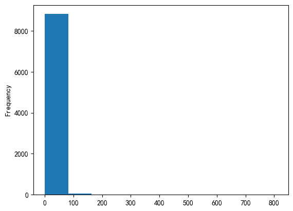
用户购买次数分布:
- 这一期间每个用户支付次数
- 统计每个用户支付次数
- 使用直方图展示
步骤:
- 过滤数据:行为为支付
- 分组:根据user_id分组,groupby
- 统计:使用count方法分组
- 可视化:使用hist方法直方图显示方法直方图显示
user_bynums=pdata[pdata.behavior_type==4].groupby('user_id')['behavior_type'].count()
user_bynums.plot.hist()
<AxesSubplot: ylabel='Frequency'>
user_bynums
user_id
4913          6
6118          1
7528          6
7591         21
12645         8
             ..
142376113     1
142412247    12
142430177     5
142450275    40
142455899    13
Name: behavior_type, Length: 8886, dtype: int64
用户复购
- 复购:用户两天以上有购买行为
复购率:复购行为用户数/有购买行为的用户总数
#实现方式1
#根据用户与时间分组,并查看数据
redata =pdata[pdata.behavior_type==4].groupby(['user_id', 'day']).count()
redata
| item_id | behavior_type | user_geohash | item_category | time | ts | hour | ||
|---|---|---|---|---|---|---|---|---|
| user_id | day | |||||||
| 4913 | 2014-12-01 | 1 | 1 | 0 | 1 | 1 | 1 | 1 |
| 2014-12-07 | 2 | 2 | 2 | 2 | 2 | 2 | 2 | |
| 2014-12-11 | 1 | 1 | 0 | 1 | 1 | 1 | 1 | |
| 2014-12-13 | 1 | 1 | 0 | 1 | 1 | 1 | 1 | |
| 2014-12-16 | 1 | 1 | 0 | 1 | 1 | 1 | 1 | |
| ... | ... | ... | ... | ... | ... | ... | ... | ... |
| 142455899 | 2014-11-24 | 1 | 1 | 0 | 1 | 1 | 1 | 1 |
| 2014-11-26 | 2 | 2 | 0 | 2 | 2 | 2 | 2 | |
| 2014-11-30 | 1 | 1 | 0 | 1 | 1 | 1 | 1 | |
| 2014-12-03 | 1 | 1 | 0 | 1 | 1 | 1 | 1 | |
| 2014-12-04 | 2 | 2 | 0 | 2 | 2 | 2 | 2 |
49201 rows × 7 columns
#重置索引
redata = redata.reset_index()
redata
| user_id | day | item_id | behavior_type | user_geohash | item_category | time | ts | hour | |
|---|---|---|---|---|---|---|---|---|---|
| 0 | 4913 | 2014-12-01 | 1 | 1 | 0 | 1 | 1 | 1 | 1 |
| 1 | 4913 | 2014-12-07 | 2 | 2 | 2 | 2 | 2 | 2 | 2 |
| 2 | 4913 | 2014-12-11 | 1 | 1 | 0 | 1 | 1 | 1 | 1 |
| 3 | 4913 | 2014-12-13 | 1 | 1 | 0 | 1 | 1 | 1 | 1 |
| 4 | 4913 | 2014-12-16 | 1 | 1 | 0 | 1 | 1 | 1 | 1 |
| ... | ... | ... | ... | ... | ... | ... | ... | ... | ... |
| 49196 | 142455899 | 2014-11-24 | 1 | 1 | 0 | 1 | 1 | 1 | 1 |
| 49197 | 142455899 | 2014-11-26 | 2 | 2 | 0 | 2 | 2 | 2 | 2 |
| 49198 | 142455899 | 2014-11-30 | 1 | 1 | 0 | 1 | 1 | 1 | 1 |
| 49199 | 142455899 | 2014-12-03 | 1 | 1 | 0 | 1 | 1 | 1 | 1 |
| 49200 | 142455899 | 2014-12-04 | 2 | 2 | 0 | 2 | 2 | 2 | 2 |
49201 rows × 9 columns
#根据user_id分组,并统计day的数量
ret = redata.groupby('user_id')['day'].count()
ret
user_id
4913         5
6118         1
7528         6
7591         9
12645        4
            ..
142376113    1
142412247    7
142430177    5
142450275    8
142455899    7
Name: day, Length: 8886, dtype: int64
#获取数量大于1的数据,计算复购率
ret[ret>1].count()/ret.count()
0.8717083051991897
#实现方式2
#根据user_id分组
re_data=pdata[pdata.behavior_type==4].groupby('user_id')
re_data
<pandas.core.groupby.generic.DataFrameGroupBy object at 0x000001D4D067CA50>
'''
使用apply方法对分组数据进行处理,
每个apply方法处理的user_id对应的series对象
使用unique获取唯一值
使用len方法获取长度
'''
re_data = re_data['day'].apply(lambda x:len(x.unique()))
re_data
user_id
4913         5
6118         1
7528         6
7591         9
12645        4
            ..
142376113    1
142412247    7
142430177    5
142450275    8
142455899    7
Name: day, Length: 8886, dtype: int64
#计算复购率
re_data[re_data>1].count()/re_data.count()
0.8717083051991897
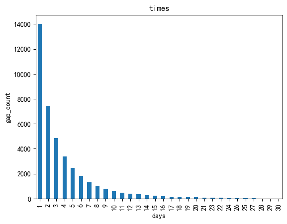
用户复购时间间隔
复购间隔:
- 按时间排序
- 用户第1次购物时间:day1
- 用户第2次购物时间:day2 , 间隔:day2-day1
- 用户第3次购物时间:day3 , 间隔:day3-day2
- 用户第N次购物时间:dayn , 间隔:dayn-dayn-1
要求:时间间隔大于0间间隔大于0
p = pd.Series([1,2,7,4,10])
p.diff(1)
0    NaN
1    1.0
2    5.0
3   -3.0
4    6.0
dtype: float64
#删除缺省值
p.diff(2).dropna()
2    6.0
3    2.0
4    3.0
dtype: float64
#分组
userbuy=pdata[pdata.behavior_type==4].groupby('user_id')
#对天进行处理
#lambda的每个x为分组后的series对象
# series对象排序,并使用diff方法计算,并去除缺省值
day_interval = userbuy.day.apply(lambda x:x.sort_values().diff(1).dropna())
C:\Users\26822\AppData\Local\Temp\ipykernel_22972\2976211149.py:6: FutureWarning: The behavior of array concatenation with empty entries is deprecated. In a future version, this will no longer exclude empty items when determining the result dtype. To retain the old behavior, exclude the empty entries before the concat operation.
  day_interval = userbuy.day.apply(lambda x:x.sort_values().diff(1).dropna())
day_interval
user_id
4913       7829893    6 days
           10689246   0 days
           11629048   4 days
           3285878    2 days
           11629584   3 days
                       ...
142455899  6697898    0 days
           9798799    4 days
           6698066    3 days
           1345137    1 days
           7372987    0 days
Name: day, Length: 111319, dtype: timedelta64[ns]
day_interval=day_interval.map(lambda x:x.days)
day_interval
user_id
4913       7829893     6
           10689246    0
           11629048    4
           3285878     2
           11629584    3
                      ..
142455899  6697898     0
           9798799     4
           6698066     3
           1345137     1
           7372987     0
Name: day, Length: 111319, dtype: int64
day_interval = day_interval[day_interval>0]
day_interval
user_id
4913       7829893     6
           11629048    4
           3285878     2
           11629584    3
7528       9688333     4
                      ..
142455899  6698002     2
           4209399     2
           9798799     4
           6698066     3
           1345137     1
Name: day, Length: 40315, dtype: int64
#统计每个时间数量,并绘制柱状图
day_interval.value_counts().plot(kind='bar')
plt.title('times')
plt.xlabel('days')
_ = plt.ylabel('gap_count')
#用户购物行为及分组
#时间间隔大于1天
day_interval = pdata[pdata.behavior_type == 4].groupby('user_id').day.apply(lambda x:x.sort_values().diff(1).dropna())
#获取天数
day_interval = day_interval.map(lambda x:x.days)
#统计数量,并绘制柱状图
day_interval.value_counts().plot(kind='bar')
plt.title('times')
plt.xlabel('days')
_ = plt.ylabel('interval_count')
C:\Users\26822\AppData\Local\Temp\ipykernel_22972\1184355078.py:3: FutureWarning: The behavior of array concatenation with empty entries is deprecated. In a future version, this will no longer exclude empty items when determining the result dtype. To retain the old behavior, exclude the empty entries before the concat operation.
  day_interval = pdata[pdata.behavior_type == 4].groupby('user_id').day.apply(lambda x:x.sort_values().diff(1).dropna())

AARRR模型
- Acquisition 用户获取
- Activation 用户激活
- Retention 提高留存
- Revenue 增加收入
- Referral 传播推荐
AARRR模型描述了用户/客户/访客需经历的五个环节,以便企业获取价值。
关键点:通过模型提高留存和转化率
- 获取用户:获取用户方式,获取用户渠道,获取用户成本,用户定位等,例如:应用下载量,安装量,注册量
- 活跃度:日活,月活,使用时长,启动次数等
- 留存率:次日留存,周留存率,不同邻域用户,留存周期不同,例如:微博,1周未登录,可以视为流失用户;
- 收入:APA(活跃付费用户数),ARPU(平均每用户收入), ARPPU(平均每付费用户收入);提高活跃度、提高留存率是增加收入基础。
- 传播推荐:用户自发传播,例如平多多砍价,核心:产品过硬:产品过硬率
event_type_count = pdata.groupby('behavior_type').size()
#重置索引并修改列名
event_type_count = event_type_count.reset_index().rename(columns={0:'total'})
#重置索引
event_type_count = event_type_count.set_index('behavior_type')
event_type_count
| total | |
|---|---|
| behavior_type | |
| 1 | 11550581 |
| 2 | 242556 |
| 3 | 343564 |
| 4 | 120205 |
# 将层级1视为基准
event_type_count['pre'] = (event_type_count.total/event_type_count.total[1])*100
event_type_count
| total | pre | |
|---|---|---|
| behavior_type | ||
| 1 | 11550581 | 100.000000 |
| 2 | 242556 | 2.099946 |
| 3 | 343564 | 2.974430 |
| 4 | 120205 | 1.040684 |
| 字段 | 字段说明 | 提取说明 |
|---|---|---|
| user_id | 用户标识 | 抽样&字段脱敏(非真实ID) |
| item_id | 商品标识 | 字段脱敏(非真实ID) |
| behavior_type | 用户对商品的行为类型 | 包括浏览、收藏、加购物车、购买,对应取值分别是1、2、3、4。 |
| user_geohash | 用户位置的空间标识,可以为空 | 由经纬度通过保密的算法生成 |
| item_category | 商品分类标识 | 字段脱敏 |
| time | 行为时间 | 精确到小时级别 |
3 用户价值分析
RFM模型是衡量当前用户价值和客户潜在价值的重要工具和手段
- R:最近一次消费(Recency)
- F:消费频率(Frequency)
- M:消费金额(Monetary)
3.1 R理解:
- 用户最近一次消费
- R值越小,说明用户的价值越高,例如:最近一次消费1个月,最近一次消费10个月
- R值非常大,说明该用户可能为流失用户;
3.2 F理解:
- 消费频率,指定时间内购买次数;
- 问题:一些商品购买频次较低,所以会将时间忽略,以购买次数为主;
- 不同品类产品,对F的理解不一样;例如:电子类产品频率较低;化妆品,衣服等消费品购买频次较高
3.3 M理解:
- 一定时间范围内,用户消费金额,消费金额越大,价值越高3.3 M理解:
#计算R,最近购物时间
#排序
tmp = pdata.sort_values('day')
#过滤数据,只保留购物的数据
tmp = tmp[tmp['behavior_type']==4]
#保留最后一个值,生成bool索引,删除最后一个,对应值为Flase
tindex = tmp.duplicated(subset=['user_id'], keep='last')
#boolean索引变化, 将False设置为True
sindex = tindex == False
#获取过滤后数据
tdata = tmp[sindex]
tdata
| user_id | item_id | behavior_type | user_geohash | item_category | time | ts | hour | day | |
|---|---|---|---|---|---|---|---|---|---|
| 6946622 | 49598175 | 176268691 | 4 | 97rjjab | 11270 | 2014-11-18 18 | 2014-11-18 18:00:00 | 18 | 2014-11-18 |
| 7917659 | 141878326 | 379814689 | 4 | NaN | 8095 | 2014-11-18 11 | 2014-11-18 11:00:00 | 11 | 2014-11-18 |
| 7549224 | 61454609 | 134625812 | 4 | 99ui5e6 | 12067 | 2014-11-18 19 | 2014-11-18 19:00:00 | 19 | 2014-11-18 |
| 10056408 | 86985041 | 105821300 | 4 | NaN | 6669 | 2014-11-18 10 | 2014-11-18 10:00:00 | 10 | 2014-11-18 |
| 1961858 | 112485959 | 228534873 | 4 | NaN | 292 | 2014-11-18 11 | 2014-11-18 11:00:00 | 11 | 2014-11-18 |
| ... | ... | ... | ... | ... | ... | ... | ... | ... | ... |
| 319576 | 131514258 | 281172663 | 4 | NaN | 1514 | 2014-12-18 10 | 2014-12-18 10:00:00 | 10 | 2014-12-18 |
| 11888591 | 123848007 | 106982400 | 4 | 956k2js | 11750 | 2014-12-18 14 | 2014-12-18 14:00:00 | 14 | 2014-12-18 |
| 3227167 | 49871598 | 47827433 | 4 | 96kajt4 | 2631 | 2014-12-18 11 | 2014-12-18 11:00:00 | 11 | 2014-12-18 |
| 6696914 | 136470861 | 347836659 | 4 | 9rf42od | 10472 | 2014-12-18 10 | 2014-12-18 10:00:00 | 10 | 2014-12-18 |
| 8618913 | 81958592 | 332303278 | 4 | 9r5frl3 | 13288 | 2014-12-18 17 | 2014-12-18 17:00:00 | 17 | 2014-12-18 |
8886 rows × 9 columns
#数量
len(tmp.groupby('user_id'))
8886
pd.to_datetime(tdata['day'])
6946622    2014-11-18
7917659    2014-11-18
7549224    2014-11-18
10056408   2014-11-18
1961858    2014-11-18
              ...
319576     2014-12-18
11888591   2014-12-18
3227167    2014-12-18
6696914    2014-12-18
8618913    2014-12-18
Name: day, Length: 8886, dtype: datetime64[ns]
tdl = pd.to_datetime('2014-12-20') - pd.to_datetime(tdata['day'])
tdata['tdays'] = tdl.dt.days
tdata
SettingWithCopyWarning:
A value is trying to be set on a copy of a slice from a DataFrame.
Try using .loc[row_indexer,col_indexer] = value instead

See the caveats in the documentation: https://pandas.pydata.org/pandas-docs/stable/user_guide/indexing.html#returning-a-view-versus-a-copy
  tdata['tdays'] = tdl.dt.days
| user_id | item_id | behavior_type | user_geohash | item_category | time | ts | hour | day | tdays | |
|---|---|---|---|---|---|---|---|---|---|---|
| 6946622 | 49598175 | 176268691 | 4 | 97rjjab | 11270 | 2014-11-18 18 | 2014-11-18 18:00:00 | 18 | 2014-11-18 | 32 |
| 7917659 | 141878326 | 379814689 | 4 | NaN | 8095 | 2014-11-18 11 | 2014-11-18 11:00:00 | 11 | 2014-11-18 | 32 |
| 7549224 | 61454609 | 134625812 | 4 | 99ui5e6 | 12067 | 2014-11-18 19 | 2014-11-18 19:00:00 | 19 | 2014-11-18 | 32 |
| 10056408 | 86985041 | 105821300 | 4 | NaN | 6669 | 2014-11-18 10 | 2014-11-18 10:00:00 | 10 | 2014-11-18 | 32 |
| 1961858 | 112485959 | 228534873 | 4 | NaN | 292 | 2014-11-18 11 | 2014-11-18 11:00:00 | 11 | 2014-11-18 | 32 |
| ... | ... | ... | ... | ... | ... | ... | ... | ... | ... | ... |
| 319576 | 131514258 | 281172663 | 4 | NaN | 1514 | 2014-12-18 10 | 2014-12-18 10:00:00 | 10 | 2014-12-18 | 2 |
| 11888591 | 123848007 | 106982400 | 4 | 956k2js | 11750 | 2014-12-18 14 | 2014-12-18 14:00:00 | 14 | 2014-12-18 | 2 |
| 3227167 | 49871598 | 47827433 | 4 | 96kajt4 | 2631 | 2014-12-18 11 | 2014-12-18 11:00:00 | 11 | 2014-12-18 | 2 |
| 6696914 | 136470861 | 347836659 | 4 | 9rf42od | 10472 | 2014-12-18 10 | 2014-12-18 10:00:00 | 10 | 2014-12-18 | 2 |
| 8618913 | 81958592 | 332303278 | 4 | 9r5frl3 | 13288 | 2014-12-18 17 | 2014-12-18 17:00:00 | 17 | 2014-12-18 | 2 |
8886 rows × 10 columns
#重置索引
rdata = tdata.set_index('user_id')
#设置R值
rdata['R'] = (rdata.tdays <= rdata.tdays.mean()).astype('i')
#过滤R列
rdata = rdata[['R']]
rdata
| R | |
|---|---|
| user_id | |
| 49598175 | 0 |
| 141878326 | 0 |
| 61454609 | 0 |
| 86985041 | 0 |
| 112485959 | 0 |
| ... | ... |
| 131514258 | 1 |
| 123848007 | 1 |
| 49871598 | 1 |
| 136470861 | 1 |
| 81958592 | 1 |
8886 rows × 1 columns
#计算F
#根据user_id分组,并且根据购物时间进行数量统计
fdata = tmp.groupby(['user_id']).time.count()
#重置索引
fdata = fdata.reset_index()
fdata = fdata.set_index('user_id')
fdata.columns = ['F']
fdata.F = pd.qcut(fdata.F, 2,['0','1'])
fdata
| F | |
|---|---|
| user_id | |
| 4913 | 0 |
| 6118 | 0 |
| 7528 | 0 |
| 7591 | 1 |
| 12645 | 0 |
| ... | ... |
| 142376113 | 0 |
| 142412247 | 1 |
| 142430177 | 0 |
| 142450275 | 1 |
| 142455899 | 1 |
8886 rows × 1 columns
# 数据集合并(R与F)
rfdata = pd.merge(rdata, fdata, left_index=True, right_index=True)
rfdata['RF'] = rfdata.R.astype(str).str.cat(rfdata.F)
rfdata
| R | F | RF | |
|---|---|---|---|
| user_id | |||
| 49598175 | 0 | 0 | 00 |
| 141878326 | 0 | 0 | 00 |
| 61454609 | 0 | 0 | 00 |
| 86985041 | 0 | 0 | 00 |
| 112485959 | 0 | 0 | 00 |
| ... | ... | ... | ... |
| 131514258 | 1 | 1 | 11 |
| 123848007 | 1 | 1 | 11 |
| 49871598 | 1 | 1 | 11 |
| 136470861 | 1 | 1 | 11 |
| 81958592 | 1 | 1 | 11 |
8886 rows × 3 columns
def func(value):
    v = '一般用户'
    if value == '00':
        v = '一般用户'
    elif value == '01':
        v = '重要保持'
    elif value == '10':
        v = '重要发展'
    elif value == '11':
        v = '重要价值'
    return v

rfdata['level'] = rfdata.RF.map(func)
rfdata
| R | F | RF | level | |
|---|---|---|---|---|
| user_id | ||||
| 49598175 | 0 | 0 | 00 | 一般用户 |
| 141878326 | 0 | 0 | 00 | 一般用户 |
| 61454609 | 0 | 0 | 00 | 一般用户 |
| 86985041 | 0 | 0 | 00 | 一般用户 |
| 112485959 | 0 | 0 | 00 | 一般用户 |
| ... | ... | ... | ... | ... |
| 131514258 | 1 | 1 | 11 | 重要价值 |
| 123848007 | 1 | 1 | 11 | 重要价值 |
| 49871598 | 1 | 1 | 11 | 重要价值 |
| 136470861 | 1 | 1 | 11 | 重要价值 |
| 81958592 | 1 | 1 | 11 | 重要价值 |
8886 rows × 4 columns
#分组统计
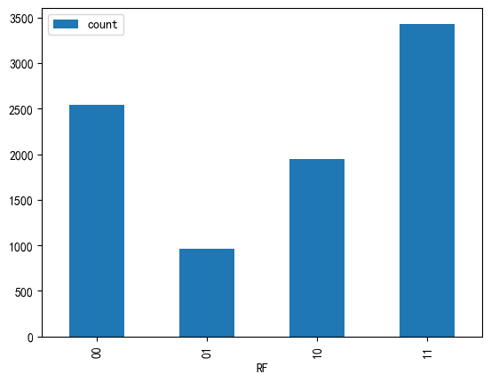
rf = rfdata.groupby('RF').F.count()
#创建DataFrame对象
rf = rf.reset_index()
#修改列名
rf = rf.rename(columns = {'F':'count'})
rf
| RF | count | |
|---|---|---|
| 0 | 00 | 2540 |
| 1 | 01 | 966 |
| 2 | 10 | 1948 |
| 3 | 11 | 3432 |
_ = rf.plot.bar(x = 'RF', y='count')