Kaggle竞赛系列_SpaceshipTitanic金牌方案分析

文章目录

- 【文章系列】
- 【前言】
- 【比赛简介】
- 【正文】
- - （一）数据获取
  - （二）数据分析
  - - 1. 缺失值
    - 2. 重复值
    - 3. 属性类型分析
    - 4. 类别分析
    - 5. 分析目标数值占比
  - （三）属性分析
  - - 1. 对年龄Age分析
    - - （1）直方图分析
      - （2）创建新属性
    - 2. 对支出属性进行分析
    - - （1）直方图分析
      - （2）创建新属性
    - 3. 对离散属性进行分析
    - - （1）直方图分析
    - 4. 对定性属性进行分析
    - - （1）属性分析
      - （2）根据PassengerId划分group
      - （3）对Cabin属性进一步划分
      - （4）根据Name的姓氏划分出家庭组
  - （四）归纳总结
  - （五）写在最后

【文章系列】

第一章初探Kaggle竞赛————Kaggle竞赛系列_Titanic比赛

第二章知识补充_随机森林————数学建模系列_随机森林

第三章知识补充_LightGBM————集成学习之Boosting方法系列_LightGBM

第四章再战Kaggle竞赛————Kaggle竞赛系列_SpaceshipTitanic比赛

第五章重温回顾_学习金牌方法_数据分析————Kaggle竞赛系列_SpaceshipTitanic金牌方案分析_数据分析

第六章重温回顾_学习金牌方法_数据处理————Kaggle竞赛系列_SpaceshipTitanic金牌方案分析_数据处理

【前言】

Spaceship Titanic比赛，类似Titanic比赛，只是增加了更多的属性以及更大的数据量，仍是一个二分类问题。

今天要分析的是一篇大神的解决方案，看完后觉得干货满满，由衷地敬佩他们对数据分析的细致程度，对比之下只觉得之前自己的分析仅仅是表面功夫，单纯靠着模型的强大能力去完成任务。看来以后还是得不断地向各位前辈大佬学习，完善自己的解决方案！！！

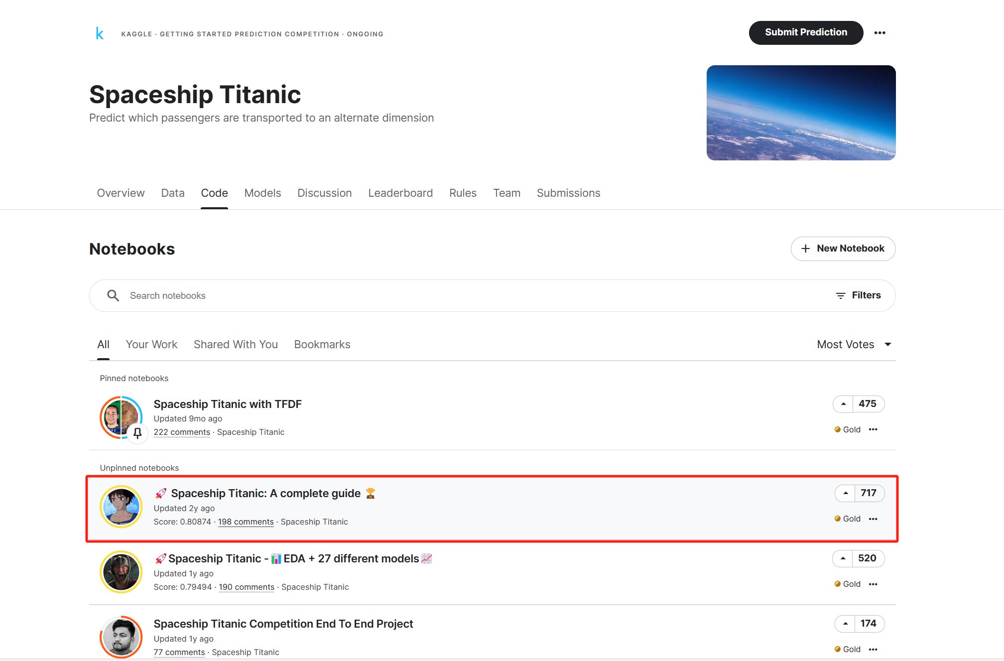
项目代码： 🚀 Spaceship Titanic: A complete guide 🏆 | Kaggle

我的解决方案：Kaggle竞赛系列_SpaceshipTitanic比赛

【比赛简介】

Spaceship Titanic比赛是一个在Kaggle上举办的机器学习挑战，参赛者的任务是预测Spaceship Titanic在与时空异常碰撞时，哪些乘客被传送到了另一个维度。这个比赛提供了从飞船损坏的计算机系统中恢复的一组个人记录，参赛者需要使用这些数据来进行预测。

【正文】

（一）数据获取

参考之前的Titanic比赛的数据获取操作 Kaggle_Titanic比赛

（二）数据分析

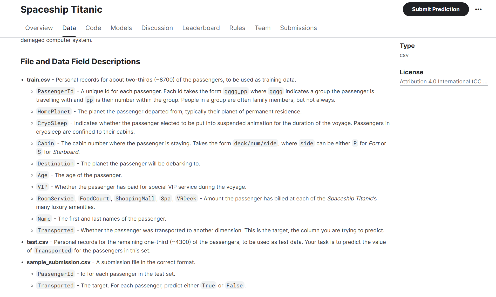
train.csv - 用于训练数据的大约三分之二（约8700名）乘客的个人记录。
PassengerId - 每位乘客的唯一标识。每个标识的格式为gggg_pp，其中gggg表示乘客所在的团体，pp是他们在团体中的编号。一个团体中的人通常是家庭成员，但并不总是如此。
HomePlanet - 乘客出发的星球，通常是他们的永久居住星球。
CryoSleep - 表示乘客是否选择在航程期间被置于悬浮动状态。处于冷冻睡眠状态的乘客被限制在他们的舱房内。
Cabin - 乘客所住的舱房号码。格式为deck/num/side，其中side可以是P（港口）或S（舷侧）。
Destination - 乘客将要下船的星球。
Age - 乘客的年龄。
VIP - 乘客是否支付额外费用获得特殊的VIP服务。
RoomService, FoodCourt, ShoppingMall, Spa, VRDeck - 乘客在太空巨轮泰坦尼克号的许多豪华设施上的费用金额。
Name - 乘客的名字和姓氏。
Transported - 乘客是否被传送到另一个维度。这是目标，也就是您要预测的列。
test.csv - 剩余三分之一（约4300名）乘客的个人记录，用作测试数据。您的任务是预测这一集合中乘客的Transported值。
sample_submission.csv - 一个以正确格式的提交文件。
PassengerId - 测试集中每位乘客的标识。
Transported - 目标。对于每位乘客，预测True或False。

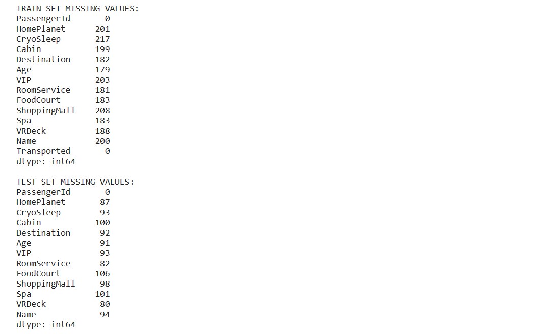
1. 缺失值

print('TRAIN SET MISSING VALUES:')
print(train.isna().sum())
print('')
print('TEST SET MISSING VALUES:')
print(test.isna().sum())

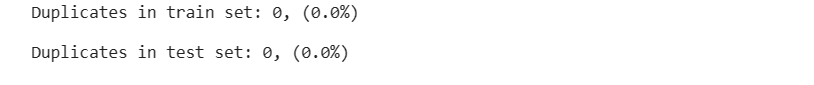
2. 重复值

print(f'Duplicates in train set: {train.duplicated().sum()}, ({np.round(100*train.duplicated().sum()/len(train),1)}%)')
print('')
print(f'Duplicates in test set: {test.duplicated().sum()}, ({np.round(100*test.duplicated().sum()/len(test),1)}%)')

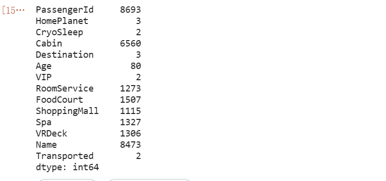
3. 属性类型分析

train.nunique()

4. 类别分析

train.dtypes

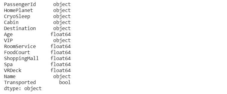
一般而言，连续型属性被存储为float和double类型，离散型属性被存储为object和int类型。

6个连续性属性(RoomService,FoodCourt,ShoppingMall,Spa,VRDeck,Age)
4个离散属性(HomePlanet,CryoSleep,Destination,VIP)
剩余3个描述性/定性属性(PassengerId,Name,Cabin)

5. 分析目标数值占比

# 特征尺寸
plt.figure(figsize=(6,6))

# 饼状图
train['Transported'].value_counts().plot.pie(explode=[0.1,0.1], autopct='%1.1f%%', shadow=True, textprops={'fontsize':16}).set_title("Target distribution")

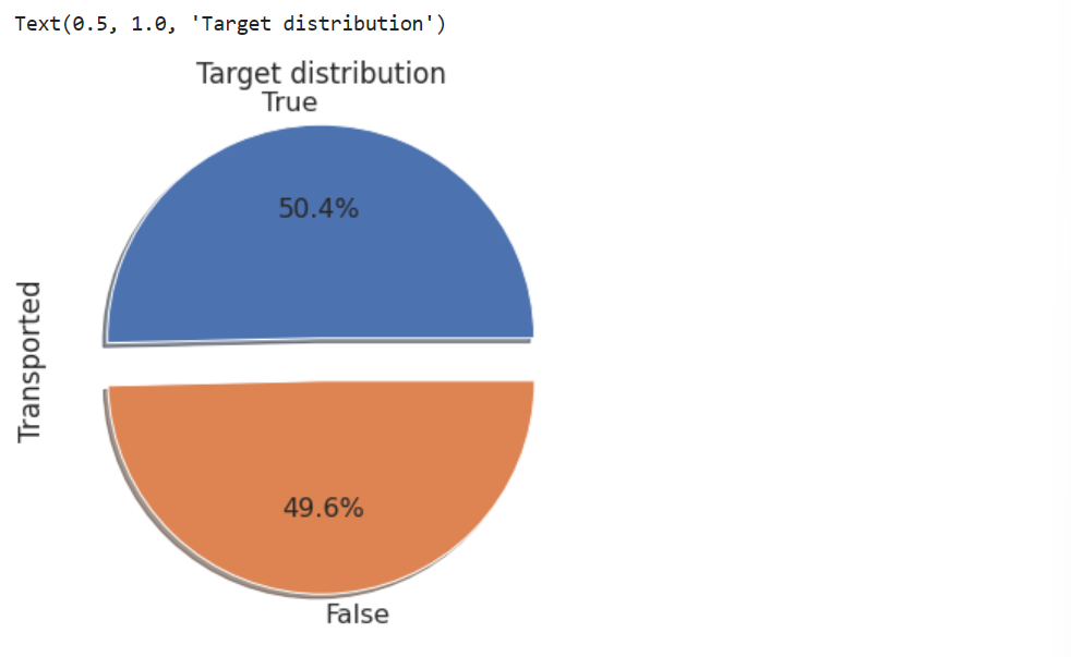
分布平衡，因此不需要采用过采样、欠采样方法。

（三）属性分析

1. 对年龄Age分析

（1）直方图分析

直方图关键参数：hue=Target属性

# 特征尺寸
plt.figure(figsize=(10,4))

# 直方图
sns.histplot(data=train, x='Age', hue='Transported', binwidth=1, kde=True)

plt.title('Age distribution')
plt.xlabel('Age (years)')

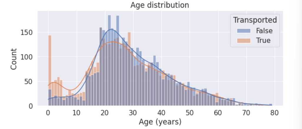
注意到：

0-18岁的青少年更容易被转移。
18-25岁的人被转移的可能性比不被转移的可能性要小。
25岁以上的人被转移的可能性和没有被转移的可能性差不多。

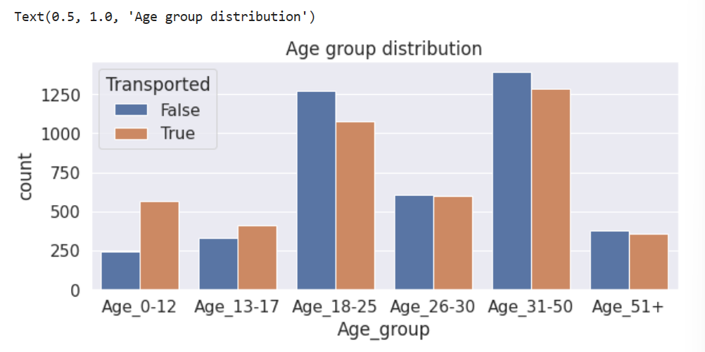
（2）创建新属性

根据直方图False与True的高度关系，对年龄划分为多层，并依次建立一个新特征。

# 新特征-训练集
train['Age_group']=np.nan
train.loc[train['Age']<=12,'Age_group']='Age_0-12'
train.loc[(train['Age']>12) & (train['Age']<18),'Age_group']='Age_13-17'
train.loc[(train['Age']>=18) & (train['Age']<=25),'Age_group']='Age_18-25'
train.loc[(train['Age']>25) & (train['Age']<=30),'Age_group']='Age_26-30'
train.loc[(train['Age']>30) & (train['Age']<=50),'Age_group']='Age_31-50'
train.loc[train['Age']>50,'Age_group']='Age_51+'

# 新特征-测试集
test['Age_group']=np.nan
test.loc[test['Age']<=12,'Age_group']='Age_0-12'
test.loc[(test['Age']>12) & (test['Age']<18),'Age_group']='Age_13-17'
test.loc[(test['Age']>=18) & (test['Age']<=25),'Age_group']='Age_18-25'
test.loc[(test['Age']>25) & (test['Age']<=30),'Age_group']='Age_26-30'
test.loc[(test['Age']>30) & (test['Age']<=50),'Age_group']='Age_31-50'
test.loc[test['Age']>50,'Age_group']='Age_51+'

# 新特征的分布图
plt.figure(figsize=(10,4))
g=sns.countplot(data=train, x='Age_group', hue='Transported', order=['Age_0-12','Age_13-17','Age_18-25','Age_26-30','Age_31-50','Age_51+'])
plt.title('Age group distribution')

2. 对支出属性进行分析

（1）直方图分析

# 支出特征
exp_feats=['RoomService', 'FoodCourt', 'ShoppingMall', 'Spa', 'VRDeck']

# 绘图
fig=plt.figure(figsize=(10,20))
for i, var_name in enumerate(exp_feats):
    # 左图
    ax=fig.add_subplot(5,2,2*i+1)
    sns.histplot(data=train, x=var_name, axes=ax, bins=30, kde=False, hue='Transported')
    ax.set_title(var_name)
    
    # 右图（核密度估计）
    ax=fig.add_subplot(5,2,2*i+2)
    sns.histplot(data=train, x=var_name, axes=ax, bins=30, kde=True, hue='Transported')
    plt.ylim([0,100])
    ax.set_title(var_name)
fig.tight_layout()  # 改善外观
plt.show()

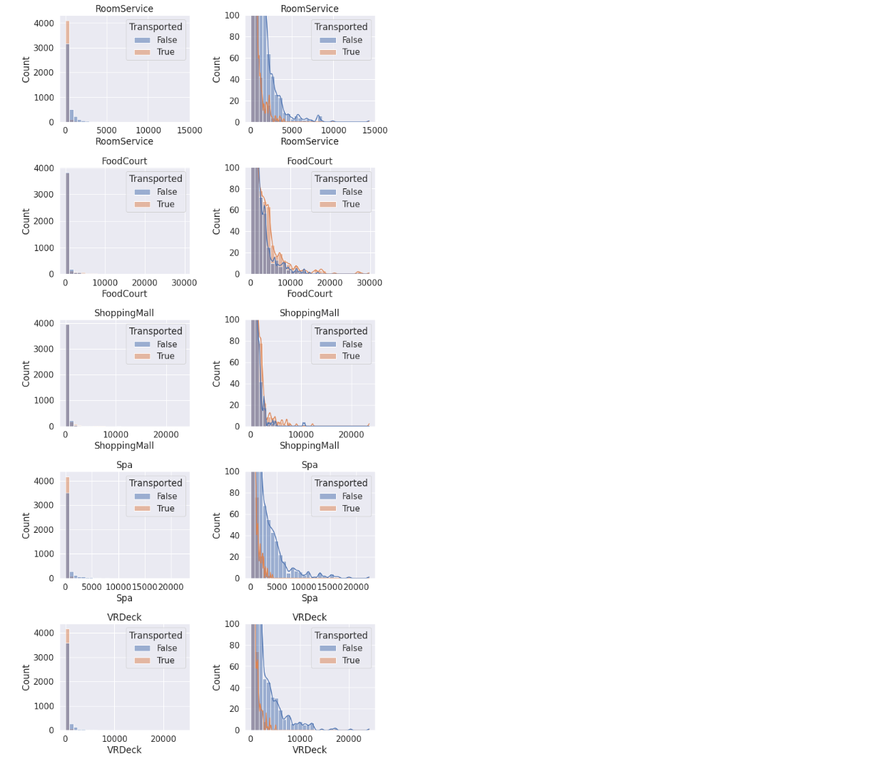
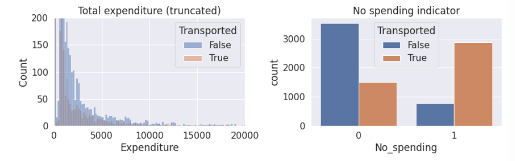
注意到：

大多数人都没有花钱，因此可以创建一个二元属性对是否有支出进行划分。
有少数的异常值。
被运输的人往往花费更少。
RoomService、Spa和VRDeck与FoodCourt和ShoppingMall有着不同的分布

（2）创建新属性

创建一个新属性记录5个支出属性的总开支。再创建一个二元属性对是否有支出进行划分。

# 新特征-训练集
train['Expenditure']=train[exp_feats].sum(axis=1)
train['No_spending']=(train['Expenditure']==0).astype(int)

# 新特征-测试集
test['Expenditure']=test[exp_feats].sum(axis=1)
test['No_spending']=(test['Expenditure']==0).astype(int)

# 新特征的分布图
fig=plt.figure(figsize=(12,4))
plt.subplot(1,2,1)
sns.histplot(data=train, x='Expenditure', hue='Transported', bins=200)
plt.title('Total expenditure (truncated)')
plt.ylim([0,200])
plt.xlim([0,20000])

plt.subplot(1,2,2)
sns.countplot(data=train, x='No_spending', hue='Transported')
plt.title('No spending indicator')
fig.tight_layout()

3. 对离散属性进行分析

（1）直方图分析

离散属性——>countplot

# 离散特征
cat_feats=['HomePlanet', 'CryoSleep', 'Destination', 'VIP']

# 绘图
fig=plt.figure(figsize=(10,16))
for i, var_name in enumerate(cat_feats):
    ax=fig.add_subplot(4,1,i+1)
    sns.countplot(data=train, x=var_name, axes=ax, hue='Transported')
    ax.set_title(var_name)
fig.tight_layout()  # 改善外观
plt.show()

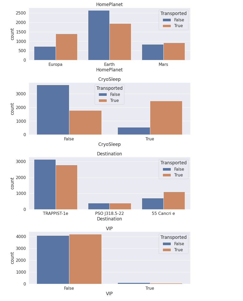
注意到：

VIP似乎不是一个有用的功能，对目标分割差不多相等。相比之下，CryoSleep似乎是一个非常有用的功能。因此我们可以考虑去掉VIP列以防止过拟合。

4. 对定性属性进行分析

（1）属性分析

# 定性特征
qual_feats=['PassengerId', 'Cabin' ,'Name']

# 预览定性特征
train[qual_feats].head()

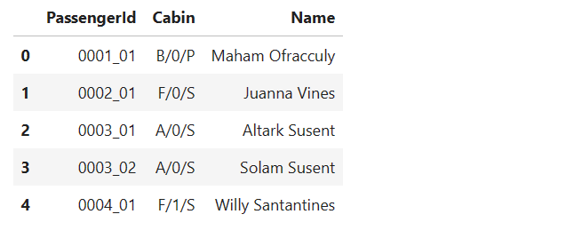
注意到：

Passengerld采用gggg_pp的形式，其中gggg表示乘客所在的旅行团，pp表示他们在旅行团中的编号。
Cabin的形式为deck/num/side，其中side可以是P代表左舷，也可以是S代表右舷。

因此我们可以从Passengerld特征中提取群组和群组大小。从Cabin特征中提取甲板、数量和侧面。从Name特征中提取姓氏来识别家庭。

（2）根据PassengerId划分group

# 新特征-分组
train['Group'] = train['PassengerId'].apply(lambda x: x.split('_')[0]).astype(int)
test['Group'] = test['PassengerId'].apply(lambda x: x.split('_')[0]).astype(int)

# 绘图
plt.figure(figsize=(20,4))
plt.subplot(1,2,1)
sns.histplot(data=train, x='Group', hue='Transported', binwidth=1)
plt.title('Group')

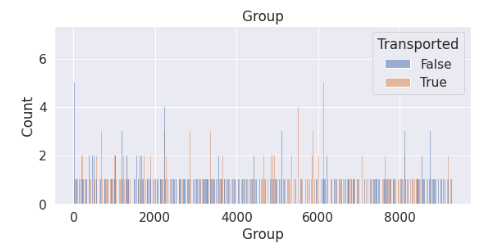
发现分组过多，不好进行独热编码，因此新建一个属性根据分组的人数记录每个分组的数量。

# 新特征-分组大小
train['Group_size']=train['Group'].map(lambda x: pd.concat([train['Group'], test['Group']]).value_counts()[x])
test['Group_size']=test['Group'].map(lambda x: pd.concat([train['Group'], test['Group']]).value_counts()[x])


plt.subplot(1,2,2)
sns.countplot(data=train, x='Group_size', hue='Transported')
plt.title('Group size')
fig.tight_layout()

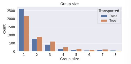
发现除了1人组更不容易被传输，其他人数的分组基本上都是更容易被传输，因此可以将其他人数的分组划分在一起。为此我们可以再新建一个属性来判断该数据是否是1人组（是否独自出行）。

# 新特征
train['Solo']=(train['Group_size']==1).astype(int)
test['Solo']=(test['Group_size']==1).astype(int)

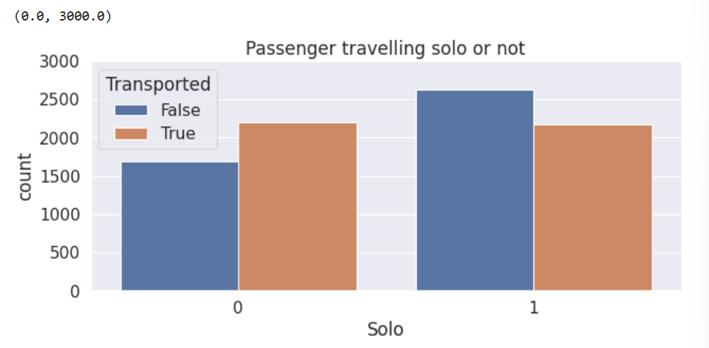
# 新特质分布图
plt.figure(figsize=(10,4))
sns.countplot(data=train, x='Solo', hue='Transported')
plt.title('Passenger travelling solo or not')
plt.ylim([0,3000])

（3）对Cabin属性进一步划分

# 现在用离群值替换NaN(这样我们就可以拆分特征)
train['Cabin'].fillna('Z/9999/Z', inplace=True)
test['Cabin'].fillna('Z/9999/Z', inplace=True)

#  新特征-训练集
train['Cabin_deck'] = train['Cabin'].apply(lambda x: x.split('/')[0])
train['Cabin_number'] = train['Cabin'].apply(lambda x: x.split('/')[1]).astype(int)
train['Cabin_side'] = train['Cabin'].apply(lambda x: x.split('/')[2])

#  新特征-测试集
test['Cabin_deck'] = test['Cabin'].apply(lambda x: x.split('/')[0])
test['Cabin_number'] = test['Cabin'].apply(lambda x: x.split('/')[1]).astype(int)
test['Cabin_side'] = test['Cabin'].apply(lambda x: x.split('/')[2])

# 把Nan的放回去(我们稍后会填充这些)
train.loc[train['Cabin_deck']=='Z', 'Cabin_deck']=np.nan
train.loc[train['Cabin_number']==9999, 'Cabin_number']=np.nan
train.loc[train['Cabin_side']=='Z', 'Cabin_side']=np.nan
test.loc[test['Cabin_deck']=='Z', 'Cabin_deck']=np.nan
test.loc[test['Cabin_number']==9999, 'Cabin_number']=np.nan
test.loc[test['Cabin_side']=='Z', 'Cabin_side']=np.nan

# 丢弃Cabin属性(我们不再需要它了)
train.drop('Cabin', axis=1, inplace=True)
test.drop('Cabin', axis=1, inplace=True)

# 新特征的分布图
fig=plt.figure(figsize=(10,12))
plt.subplot(3,1,1)
sns.countplot(data=train, x='Cabin_deck', hue='Transported', order=['A','B','C','D','E','F','G','T'])
plt.title('Cabin deck')

plt.subplot(3,1,2)
sns.histplot(data=train, x='Cabin_number', hue='Transported',binwidth=20)
plt.vlines(300, ymin=0, ymax=200, color='black')
plt.vlines(600, ymin=0, ymax=200, color='black')
plt.vlines(900, ymin=0, ymax=200, color='black')
plt.vlines(1200, ymin=0, ymax=200, color='black')
plt.vlines(1500, ymin=0, ymax=200, color='black')
plt.vlines(1800, ymin=0, ymax=200, color='black')
plt.title('Cabin number')
plt.xlim([0,2000])

plt.subplot(3,1,3)
sns.countplot(data=train, x='Cabin_side', hue='Transported')
plt.title('Cabin side')
fig.tight_layout()

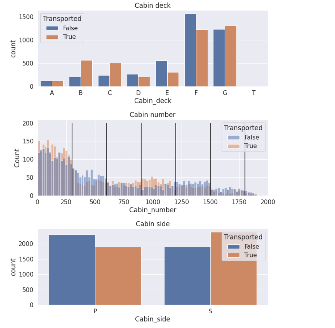
注意到Cabin_number被按照300的数量进行划分，每个划分的False与True的高度都不一样。这意味着我们可以压缩这个特征被压缩成一个分类特征，其他注意事项:客舱甲板的“T”似乎是一个异常值(只有5个样本)。

# 新特征-训练集
train['Cabin_region1']=(train['Cabin_number']<300).astype(int)   # 独热编码
train['Cabin_region2']=((train['Cabin_number']>=300) & (train['Cabin_number']<600)).astype(int)
train['Cabin_region3']=((train['Cabin_number']>=600) & (train['Cabin_number']<900)).astype(int)
train['Cabin_region4']=((train['Cabin_number']>=900) & (train['Cabin_number']<1200)).astype(int)
train['Cabin_region5']=((train['Cabin_number']>=1200) & (train['Cabin_number']<1500)).astype(int)
train['Cabin_region6']=((train['Cabin_number']>=1500) & (train['Cabin_number']<1800)).astype(int)
train['Cabin_region7']=(train['Cabin_number']>=1800).astype(int)

# 新特征-测试集
test['Cabin_region1']=(test['Cabin_number']<300).astype(int)   # 独热编码
test['Cabin_region2']=((test['Cabin_number']>=300) & (test['Cabin_number']<600)).astype(int)
test['Cabin_region3']=((test['Cabin_number']>=600) & (test['Cabin_number']<900)).astype(int)
test['Cabin_region4']=((test['Cabin_number']>=900) & (test['Cabin_number']<1200)).astype(int)
test['Cabin_region5']=((test['Cabin_number']>=1200) & (test['Cabin_number']<1500)).astype(int)
test['Cabin_region6']=((test['Cabin_number']>=1500) & (test['Cabin_number']<1800)).astype(int)
test['Cabin_region7']=(test['Cabin_number']>=1800).astype(int)

# 新特征的分布图
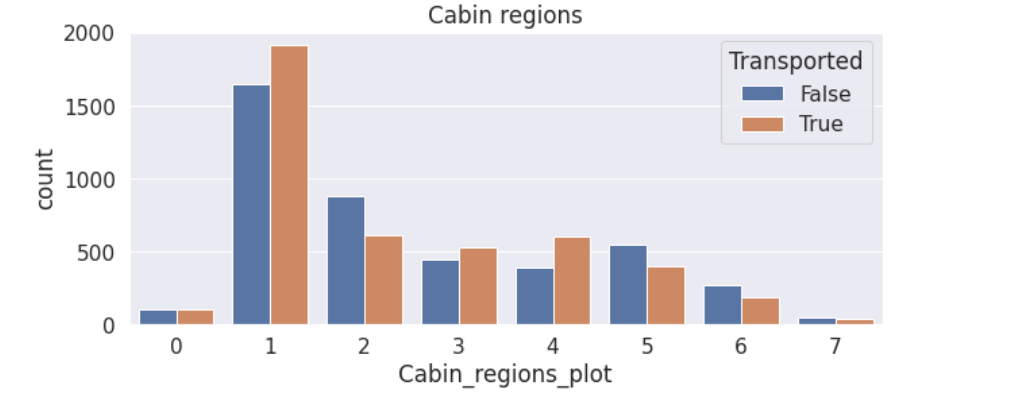
plt.figure(figsize=(10,4))
train['Cabin_regions_plot']=(train['Cabin_region1']+2*train['Cabin_region2']+3*train['Cabin_region3']+4*train['Cabin_region4']+5*train['Cabin_region5']+6*train['Cabin_region6']+7*train['Cabin_region7']).astype(int)
sns.countplot(data=train, x='Cabin_regions_plot', hue='Transported')
plt.title('Cabin regions')
train.drop('Cabin_regions_plot', axis=1, inplace=True)

（4）根据Name的姓氏划分出家庭组

根据形式划分出家庭组，再根据家庭组的大小划分出一个新的二元属性。

# 现在用离群值替换NaN(这样我们就可以拆分特征)
train['Name'].fillna('Unknown Unknown', inplace=True)
test['Name'].fillna('Unknown Unknown', inplace=True)

# 新特征-姓氏
train['Surname']=train['Name'].str.split().str[-1]
test['Surname']=test['Name'].str.split().str[-1]

# 新特征-家庭大小
train['Family_size']=train['Surname'].map(lambda x: pd.concat([train['Surname'],test['Surname']]).value_counts()[x])
test['Family_size']=test['Surname'].map(lambda x: pd.concat([train['Surname'],test['Surname']]).value_counts()[x])

# 把Nan的放回去(我们稍后会填充这些)
train.loc[train['Surname']=='Unknown','Surname']=np.nan
train.loc[train['Family_size']>100,'Family_size']=np.nan
test.loc[test['Surname']=='Unknown','Surname']=np.nan
test.loc[test['Family_size']>100,'Family_size']=np.nan

# 删除Name(我们不再需要它了)
train.drop('Name', axis=1, inplace=True)
test.drop('Name', axis=1, inplace=True)

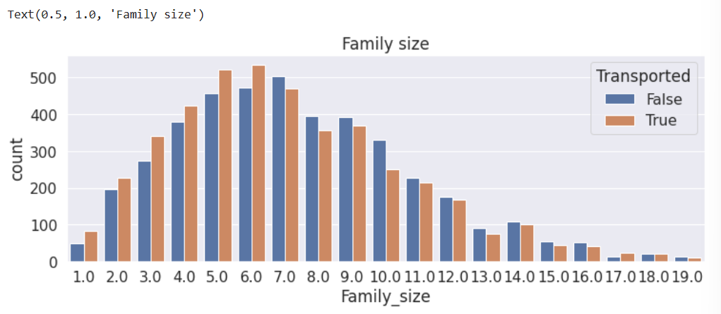
# 新特征分布图
plt.figure(figsize=(12,4))
sns.countplot(data=train, x='Family_size', hue='Transported')
plt.title('Family size')