文章目录
- Pandas分析练习题
- 1. 获取并了解数据
- 2. 数据过滤与排序
- 3. 数据分组
- 4. Apply函数
- 5. 合并数据
- 6. 数据统计
- 7. 数据可视化
- 8. 创建数据框
- 9. 时间序列
- 10. 删除数据
代码均在Jupter Notebook上完成
Pandas分析练习题
-
数据集可从此获取:
链接: https://pan.baidu.com/s/1YGwh3pqxW4OlrQXt-5wgFg?pwd=3znx 提取码: 3znx
| 简介 | 数据集 |
|---|---|
| 1.分析Chipotle快餐数据 | chipotle.tsv |
| 2.分析2012欧洲杯数据 | Euro2012_stats.csv |
| 3.分析酒类消费数据 | drinks.csv |
| 4.分析1960 - 2014 美国犯罪数据 | US_Crime_Rates_1960_2014.csv |
| 5.分析虚拟姓名数据 | 题内构造数据 |
| 6.分析风速数据 | wind.data |
| 7.分析泰坦尼克灾难数据 | train.csv |
| 8.分析Pokemon数据 | 练习中手动内置的数据 |
| 9.分析Apple公司股价数据 | Apple_stock.csv |
| 10.分析Iris纸鸢花数据 | iris.csv |
1. 获取并了解数据
import pandas as pd
csv_path='./pandas_data/chipotle.tsv'
#1.加载数据
chipo=pd.read_csv(csv_path,sep='\t')
#2.查看数据的前10行
print(chipo.head(10))
print('----------1----------')
#3.查看数据有多少列
print(chipo.shape[1])
print('----------2----------')
#4.打印全部列名
print(chipo.columns)
print('----------3----------')
#5. 查看数据集索引
print(chipo.index)
print('----------4----------')
#6. 查看下单数量最多的商品
c = chipo[['item_name', 'quantity']].groupby(['item_name'], as_index=False).agg({'quantity': sum})
c.sort_values(by='quantity',ascending=False,inplace=True)
print(c.head(1))
print('----------5----------')

#7. 查看有多少种商品 中已经对商品名称进行去重,因此只需要记录商品名称个数即可
print(c['quantity'].count())
#7.1 方法2
print(chipo['item_name'].nunique())
print('----------6----------')
#8. 在choice_description中,下单次数最多的商品是什么?
print(chipo['choice_description'].value_counts().head(1))
print('----------7----------')
#9. 下单商品总量
print(chipo['quantity'].sum())
#10. 将价格iten_priceabs转换为浮点数
d=lambda x: float(x[1:])
chipo['item_price']=chipo['item_price'].apply(d)
print(chipo['item_price'].dtype)
print('----------8----------')
#11. 计算总收入
chipo['sub_total']=chipo['item_price']*chipo['quantity']
print(chipo['sub_total'].sum())
print('----------9----------')
# 12: 订单总量
print(chipo['order_id'].nunique())
   order_id  quantity                              item_name  \
0         1         1           Chips and Fresh Tomato Salsa
1         1         1                                   Izze
2         1         1                       Nantucket Nectar
3         1         1  Chips and Tomatillo-Green Chili Salsa
4         2         2                           Chicken Bowl
5         3         1                           Chicken Bowl
6         3         1                          Side of Chips
7         4         1                          Steak Burrito
8         4         1                       Steak Soft Tacos
9         5         1                          Steak Burrito

                                  choice_description item_price
0                                                NaN     $2.39
1                                       [Clementine]     $3.39
2                                            [Apple]     $3.39
3                                                NaN     $2.39
4  [Tomatillo-Red Chili Salsa (Hot), [Black Beans...    $16.98
5  [Fresh Tomato Salsa (Mild), [Rice, Cheese, Sou...    $10.98
6                                                NaN     $1.69
7  [Tomatillo Red Chili Salsa, [Fajita Vegetables...    $11.75
8  [Tomatillo Green Chili Salsa, [Pinto Beans, Ch...     $9.25
9  [Fresh Tomato Salsa, [Rice, Black Beans, Pinto...     $9.25
----------1----------
5
----------2----------
Index(['order_id', 'quantity', 'item_name', 'choice_description',
       'item_price'],
      dtype='object')
----------3----------
RangeIndex(start=0, stop=4622, step=1)
----------4----------
       item_name  quantity
17  Chicken Bowl       761
----------5----------
50
50
----------6----------
[Diet Coke]    134
Name: choice_description, dtype: int64
----------7----------
4972
float64
----------8----------
39237.02
1834
2. 数据过滤与排序
csv_path2="./pandas_data/Euro2012_stats.csv"
#1:加载数据
euro=pd.read_csv(csv_path2)
print(euro.head())
print('----------1----------')
#2.读取Goals列
print(euro['Goals'])
print('----------2----------')
#3.统计球队数量
print(euro.shape[0])
print('----------3----------')
#4.查看数据集信息
print(euro.info())
print('----------4----------')
#5.将Team、Yellow Cards、Red Cards单独存储到一个数据集
subset=euro[['Team','Yellow Cards','Red Cards']]
print(subset.head())
print('----------5----------')
#6. 对数据集5按Red Cards、Yellow Cards排序
sorted_subset=subset.sort_values(['Red Cards','Yellow Cards'],ascending=False)
print(sorted_subset)
print('----------6----------')
#7.计算黄牌平均值
print(round(subset['Yellow Cards'].mean()))
print('----------7----------')
#8. 找出进球数大于6的球队
print(euro[euro['Goals']>6][['Team','Goals']])
print('----------8----------')
#9. 选取G开头的球队
#方法1 contains方法加正则表达式
print(euro[euro['Team'].str.contains('^G')]['Team'])
#方法2
print(euro[euro.Team.str.startswith('G')]['Team'])
print('----------9----------')
#10. 选取前7列
print(euro.iloc[:,0:7])
#11. 选取除了最后3列之外的全部列
print(euro.iloc[:,:-3])
#12. 找到英格兰(England)、意大利(Italy)和俄罗斯(Russia)的射正率(Shooting Accuracy)
print(euro.loc[euro['Team'].isin(['England', 'Italy', 'Russia']),['Team', 'Shooting Accuracy']])
Team Goals Shots on target Shots off target Shooting Accuracy \
0 Croatia 4 13 12 51.9%
1 Czech Republic 4 13 18 41.9%
2 Denmark 4 10 10 50.0%
3 England 5 11 18 50.0%
4 France 3 22 24 37.9%
% Goals-to-shots Total shots (inc. Blocked) Hit Woodwork Penalty goals \
0 16.0% 32 0 0
1 12.9% 39 0 0
2 20.0% 27 1 0
3 17.2% 40 0 0
4 6.5% 65 1 0
Penalties not scored ... Saves made Saves-to-shots ratio Fouls Won \
0 0 ... 13 81.3% 41
1 0 ... 9 60.1% 53
2 0 ... 10 66.7% 25
3 0 ... 22 88.1% 43
4 0 ... 6 54.6% 36
Fouls Conceded Offsides Yellow Cards Red Cards Subs on Subs off \
0 62 2 9 0 9 9
1 73 8 7 0 11 11
2 38 8 4 0 7 7
3 45 6 5 0 11 11
4 51 5 6 0 11 11
Players Used
0 16
1 19
2 15
3 16
4 19
[5 rows x 35 columns]
----------1----------
0 4
1 4
2 4
3 5
4 3
5 10
6 5
7 6
8 2
9 2
10 6
11 1
12 5
13 12
14 5
15 2
Name: Goals, dtype: int64
----------2----------
16
----------3----------
<class 'pandas.core.frame.DataFrame'>
RangeIndex: 16 entries, 0 to 15
Data columns (total 35 columns):
# Column Non-Null Count Dtype
--- ------ -------------- -----
0 Team 16 non-null object
1 Goals 16 non-null int64
2 Shots on target 16 non-null int64
3 Shots off target 16 non-null int64
4 Shooting Accuracy 16 non-null object
5 % Goals-to-shots 16 non-null object
6 Total shots (inc. Blocked) 16 non-null int64
7 Hit Woodwork 16 non-null int64
8 Penalty goals 16 non-null int64
9 Penalties not scored 16 non-null int64
10 Headed goals 16 non-null int64
11 Passes 16 non-null int64
12 Passes completed 16 non-null int64
13 Passing Accuracy 16 non-null object
14 Touches 16 non-null int64
15 Crosses 16 non-null int64
16 Dribbles 16 non-null int64
17 Corners Taken 16 non-null int64
18 Tackles 16 non-null int64
19 Clearances 16 non-null int64
20 Interceptions 16 non-null int64
21 Clearances off line 15 non-null float64
22 Clean Sheets 16 non-null int64
23 Blocks 16 non-null int64
24 Goals conceded 16 non-null int64
25 Saves made 16 non-null int64
26 Saves-to-shots ratio 16 non-null object
27 Fouls Won 16 non-null int64
28 Fouls Conceded 16 non-null int64
29 Offsides 16 non-null int64
30 Yellow Cards 16 non-null int64
31 Red Cards 16 non-null int64
32 Subs on 16 non-null int64
33 Subs off 16 non-null int64
34 Players Used 16 non-null int64
dtypes: float64(1), int64(29), object(5)
memory usage: 4.5+ KB
None
----------4----------
Team Yellow Cards Red Cards
0 Croatia 9 0
1 Czech Republic 7 0
2 Denmark 4 0
3 England 5 0
4 France 6 0
----------5----------
Team Yellow Cards Red Cards
6 Greece 9 1
9 Poland 7 1
11 Republic of Ireland 6 1
7 Italy 16 0
10 Portugal 12 0
13 Spain 11 0
0 Croatia 9 0
1 Czech Republic 7 0
14 Sweden 7 0
4 France 6 0
12 Russia 6 0
3 England 5 0
8 Netherlands 5 0
15 Ukraine 5 0
2 Denmark 4 0
5 Germany 4 0
----------6----------
7
----------7----------
Team Goals
5 Germany 10
13 Spain 12
----------8----------
5 Germany
6 Greece
Name: Team, dtype: object
5 Germany
6 Greece
Name: Team, dtype: object
----------9----------
Team Goals Shots on target Shots off target \
0 Croatia 4 13 12
1 Czech Republic 4 13 18
2 Denmark 4 10 10
3 England 5 11 18
4 France 3 22 24
5 Germany 10 32 32
6 Greece 5 8 18
7 Italy 6 34 45
8 Netherlands 2 12 36
9 Poland 2 15 23
10 Portugal 6 22 42
11 Republic of Ireland 1 7 12
12 Russia 5 9 31
13 Spain 12 42 33
14 Sweden 5 17 19
15 Ukraine 2 7 26
Shooting Accuracy % Goals-to-shots Total shots (inc. Blocked)
0 51.9% 16.0% 32
1 41.9% 12.9% 39
2 50.0% 20.0% 27
3 50.0% 17.2% 40
4 37.9% 6.5% 65
5 47.8% 15.6% 80
6 30.7% 19.2% 32
7 43.0% 7.5% 110
8 25.0% 4.1% 60
9 39.4% 5.2% 48
10 34.3% 9.3% 82
11 36.8% 5.2% 28
12 22.5% 12.5% 59
13 55.9% 16.0% 100
14 47.2% 13.8% 39
15 21.2% 6.0% 38
Team Goals Shots on target Shots off target \
0 Croatia 4 13 12
1 Czech Republic 4 13 18
2 Denmark 4 10 10
3 England 5 11 18
4 France 3 22 24
5 Germany 10 32 32
6 Greece 5 8 18
7 Italy 6 34 45
8 Netherlands 2 12 36
9 Poland 2 15 23
10 Portugal 6 22 42
11 Republic of Ireland 1 7 12
12 Russia 5 9 31
13 Spain 12 42 33
14 Sweden 5 17 19
15 Ukraine 2 7 26
Shooting Accuracy % Goals-to-shots Total shots (inc. Blocked) \
0 51.9% 16.0% 32
1 41.9% 12.9% 39
2 50.0% 20.0% 27
3 50.0% 17.2% 40
4 37.9% 6.5% 65
5 47.8% 15.6% 80
6 30.7% 19.2% 32
7 43.0% 7.5% 110
8 25.0% 4.1% 60
9 39.4% 5.2% 48
10 34.3% 9.3% 82
11 36.8% 5.2% 28
12 22.5% 12.5% 59
13 55.9% 16.0% 100
14 47.2% 13.8% 39
15 21.2% 6.0% 38
Hit Woodwork Penalty goals Penalties not scored ... Clean Sheets \
0 0 0 0 ... 0
1 0 0 0 ... 1
2 1 0 0 ... 1
3 0 0 0 ... 2
4 1 0 0 ... 1
5 2 1 0 ... 1
6 1 1 1 ... 1
7 2 0 0 ... 2
8 2 0 0 ... 0
9 0 0 0 ... 0
10 6 0 0 ... 2
11 0 0 0 ... 0
12 2 0 0 ... 0
13 0 1 0 ... 5
14 3 0 0 ... 1
15 0 0 0 ... 0
Blocks Goals conceded Saves made Saves-to-shots ratio Fouls Won \
0 10 3 13 81.3% 41
1 10 6 9 60.1% 53
2 10 5 10 66.7% 25
3 29 3 22 88.1% 43
4 7 5 6 54.6% 36
5 11 6 10 62.6% 63
6 23 7 13 65.1% 67
7 18 7 20 74.1% 101
8 9 5 12 70.6% 35
9 8 3 6 66.7% 48
10 11 4 10 71.5% 73
11 23 9 17 65.4% 43
12 8 3 10 77.0% 34
13 8 1 15 93.8% 102
14 12 5 8 61.6% 35
15 4 4 13 76.5% 48
Fouls Conceded Offsides Yellow Cards Red Cards
0 62 2 9 0
1 73 8 7 0
2 38 8 4 0
3 45 6 5 0
4 51 5 6 0
5 49 12 4 0
6 48 12 9 1
7 89 16 16 0
8 30 3 5 0
9 56 3 7 1
10 90 10 12 0
11 51 11 6 1
12 43 4 6 0
13 83 19 11 0
14 51 7 7 0
15 31 4 5 0
[16 rows x 32 columns]
Team Shooting Accuracy
3 England 50.0%
7 Italy 43.0%
12 Russia 22.5%
3. 数据分组
csv_path3="./pandas_data/drinks.csv"
#1:加载数据
drinks=pd.read_csv(csv_path3)
print(drinks)
print('----------1----------')
#2.计算各大洲啤酒平均消耗量
print(drinks.groupby('continent')['beer_servings'].mean())
print('----------2----------')
#3.计算各大洲红酒平均消耗量
print(drinks.groupby('continent')['wine_servings'].mean())
print('----------3----------')
#4.打印出各大洲每种酒类别的消耗平均值
print(drinks.groupby('continent')['beer_servings','spirit_servings','wine_servings'].mean())
print('----------4----------')
#5.打印出各大洲每种酒类别的消耗中位数
print(drinks.groupby('continent')['beer_servings','spirit_servings','wine_servings'].median())
print('----------5----------')
#6. 打印出各大洲对spirit饮品消耗的平均值,最大值和最小值
print(drinks.groupby('continent')['spirit_servings'].agg(['mean', 'min', 'max']))
         country  beer_servings  spirit_servings  wine_servings  \
0    Afghanistan              0                0              0
1        Albania             89              132             54
2        Algeria             25                0             14
3        Andorra            245              138            312
4         Angola            217               57             45
..           ...            ...              ...            ...
188    Venezuela            333              100              3
189      Vietnam            111                2              1
190        Yemen              6                0              0
191       Zambia             32               19              4
192     Zimbabwe             64               18              4

     total_litres_of_pure_alcohol continent
0                             0.0        AS
1                             4.9        EU
2                             0.7        AF
3                            12.4        EU
4                             5.9        AF
..                            ...       ...
188                           7.7        SA
189                           2.0        AS
190                           0.1        AS
191                           2.5        AF
192                           4.7        AF

[193 rows x 6 columns]
----------1----------
continent
AF     61.471698
AS     37.045455
EU    193.777778
OC     89.687500
SA    175.083333
Name: beer_servings, dtype: float64
----------2----------
continent
AF     16.264151
AS      9.068182
EU    142.222222
OC     35.625000
SA     62.416667
Name: wine_servings, dtype: float64
----------3----------
           beer_servings  spirit_servings  wine_servings
continent
AF             61.471698        16.339623      16.264151
AS             37.045455        60.840909       9.068182
EU            193.777778       132.555556     142.222222
OC             89.687500        58.437500      35.625000
SA            175.083333       114.750000      62.416667
----------4----------
           beer_servings  spirit_servings  wine_servings
continent
AF                  32.0              3.0            2.0
AS                  17.5             16.0            1.0
EU                 219.0            122.0          128.0
OC                  52.5             37.0            8.5
SA                 162.5            108.5           12.0
----------5----------
                 mean  min  max
continent
AF          16.339623    0  152
AS          60.840909    0  326
EU         132.555556    0  373
OC          58.437500    0  254
SA         114.750000   25  302


/var/folders/cr/2fpn8__12377w89ml3mv5ksw0000gn/T/ipykernel_74870/3785898223.py:13: FutureWarning: Indexing with multiple keys (implicitly converted to a tuple of keys) will be deprecated, use a list instead.
  print(drinks.groupby('continent')['beer_servings','spirit_servings','wine_servings'].mean())
/var/folders/cr/2fpn8__12377w89ml3mv5ksw0000gn/T/ipykernel_74870/3785898223.py:16: FutureWarning: Indexing with multiple keys (implicitly converted to a tuple of keys) will be deprecated, use a list instead.
  print(drinks.groupby('continent')['beer_servings','spirit_servings','wine_servings'].median())
4. Apply函数
注意:在 Pandas 中,你可以使用 pd.to_datetime 函数将一个包含日期或时间信息的列转换为 datetime64 数据类型。
pd.to_datetime 函数用于将输入的日期、时间、字符串或类似对象转换为 Pandas 中的 datetime64[ns] 类型。以下是该函数的主要参数说明:
语法:
pd.to_datetime(arg, errors='raise', dayfirst=False, yearfirst=False, utc=None, format=None, exact=True, unit=None, infer_datetime_format=False, origin='unix', cache=False)
主要参数:
arg: 要转换的日期、时间、字符串或类似对象。
errors: 指定在转换失败时的处理方式,可以是 ‘raise’(默认,抛出异常)、‘coerce’(将无法转换的值设为 NaT)或 ‘ignore’(忽略错误)。
dayfirst: 如果为 True,解析的字符串中的日期在前,月份在后。默认为 False。
yearfirst: 如果为 True,解析的字符串中的年份在前,月份在后。默认为 False。
utc: 如果为 True,则返回的时间是 UTC 标准时间。默认为 None。
format: 指定日期字符串的格式,可以提高解析速度。如果未指定,则尝试使用通用解析器。
exact: 如果为 False,允许近似解析,例如将日期范围扩大到有效范围内。默认为 True。
unit: 控制解析结果的时间单位,可以是 ‘D’(日)、‘s’(秒)、‘ms’(毫秒)、‘us’(微秒)、‘ns’(纳秒)。
infer_datetime_format: 如果为 True,尝试推断日期字符串的格式以提高解析速度。默认为 False。
origin: 设置日期的起始点,可以是 ‘unix’(默认,1970-01-01),‘epoch’(1970-01-01),或一个具体的日期字符串。
cache: 如果为 True,则缓存解析后的日期,提高性能。默认为 False。
set_index 是 Pandas 中用于设置 DataFrame 索引的函数。该函数可以将一个或多个列设置为 DataFrame 的索引,或者通过设置 drop 参数保留原始列并将其从 DataFrame 中移除。
作用: 设置 DataFrame 的索引,可以根据指定的列或多列构建一个新的索引。
语法:
DataFrame.set_index(keys, drop=True, append=False, inplace=False, verify_integrity=False)
主要参数说明:
keys: 用于设置索引的列名,可以是单个列名或列名的列表。
drop: 如果为 True,则将设置为索引的列从 DataFrame 中删除,默认为 True。
append: 如果为 True,则将新索引添加到现有索引的末尾,形成多级索引,默认为 False。
inplace: 如果为 True,则在原地修改 DataFrame,否则返回一个新的 DataFrame,默认为 False。
verify_integrity: 如果为 True,则检查新的索引是否唯一。如果新索引中存在重复值,将引发 ValueError,默认为 False。
resample 函数是 Pandas 中用于对时间序列数据进行重新采样的重要工具。它允许你按照指定的时间频率对数据进行聚合、转换或者采样。
主要作用:
聚合和汇总: 将时间序列数据按照指定的时间频率进行分组,然后进行聚合操作,比如求和、平均值等。
转换: 可以对时间序列数据进行转换操作,例如插值、填充缺失值等。
降采样和升采样: 降采样是指将高频率的数据聚合为低频率,而升采样是指将低频率的数据转换为高频率。
语法:
DataFrame.resample(rule, how=None, axis=0, fill_method=None, closed=None, label=None, convention='start', kind=None, loffset=None, limit=None, base=0, on=None, level=None)
主要参数说明:
rule: 重新采样的规则,可以是字符串(如 ‘D’ 表示日,‘M’ 表示月)或者 Timedelta 对象。
‘D’: 每天
‘W’: 每周
‘M’: 每月
‘Q’: 每季度
‘A’: 每年
‘AS’: 每年的开始(Annual Start)
how: 聚合函数,例如 ‘sum’、‘mean’ 等。默认为 None,表示使用每个时间窗口的第一个数据。
axis: 指定要操作的轴,默认为 0。
fill_method: 用于升采样时填充缺失值的方法,比如 ‘ffill’(向前填充)或 ‘bfill’(向后填充)。
closed: 控制区间的闭合方式,‘right’ 表示右闭合,‘left’ 表示左闭合,默认为 None。
label: 控制标签的选择,可以是 ‘left’(使用左边界标签)或 ‘right’(使用右边界标签),默认为 None。
convention: 用于区间的开合方式,可以是 ‘start’(默认,表示左闭右开)或 ‘end’(表示左开右闭)。
kind: 指定采样的类型,可以是 ‘timestamp’(时间戳,默认)或 ‘period’(周期)。
loffset: 用于调整采样结果的时间偏移。
limit: 用于降采样时限制填充的连续 NaN 的个数。
base: 用于设置相对周期的基准值。
on: 用于对 DataFrame 进行按列重采样时指定用于采样的列。
level: 用于 MultiIndex 的级别。
idxmax() 是 Pandas 中的一个函数,它返回 Series 或 DataFrame 中最大值所在的索引位置。具体作用如下:
作用: 返回最大值所在的索引位置。
语法:
Series.idxmax(axis=0, skipna=True, *args, **kwargs)
axis: 用于指定轴方向,对于 Series,只能是 0;对于 DataFrame,可以是 0 或 1,默认为 0。
skipna: 控制是否忽略 NaN 值,默认为 True。
csv_path4="./pandas_data/US_Crime_Rates_1960_2014.csv"
#1:加载数据
crime=pd.read_csv(csv_path4)
print(crime.head())
print('----------1----------')
#2.查看数据集信息
print(crime.info())
print('----------2----------')
#3.将Year列数据类型转为datetime64
print(crime['Year'].dtype)
crime['Year']=pd.to_datetime(crime['Year'],format='%Y')
print(crime['Year'].dtype)
print('----------3----------')
#4.将Year设置为数据集索引
crime=crime.set_index('Year',drop=True)
print(crime.head())
print('----------4----------')
#5.删除Total列
#方法1
crime.drop('Total',axis=1,inplace=True)
#方法2
#del crime['Total']
print(crime.head())
print('----------5----------')
#6. 按照Year对数据进行分组求和
crimes=crime.resample('10AS').sum()
population = crime['Population'].resample('10AS').max()
crimes['Population'] = population
print(crimes)
print('----------6----------')
#7.  打印历史最危险的时代
print(crime.idxmax())
   Year  Population    Total  Violent  Property  Murder  Forcible_Rape  \
0  1960   179323175  3384200   288460   3095700    9110          17190
1  1961   182992000  3488000   289390   3198600    8740          17220
2  1962   185771000  3752200   301510   3450700    8530          17550
3  1963   188483000  4109500   316970   3792500    8640          17650
4  1964   191141000  4564600   364220   4200400    9360          21420

   Robbery  Aggravated_assault  Burglary  Larceny_Theft  Vehicle_Theft
0   107840              154320    912100        1855400         328200
1   106670              156760    949600        1913000         336000
2   110860              164570    994300        2089600         366800
3   116470              174210   1086400        2297800         408300
4   130390              203050   1213200        2514400         472800
----------1----------
<class 'pandas.core.frame.DataFrame'>
RangeIndex: 55 entries, 0 to 54
Data columns (total 12 columns):
 #   Column              Non-Null Count  Dtype
---  ------              --------------  -----
 0   Year                55 non-null     int64
 1   Population          55 non-null     int64
 2   Total               55 non-null     int64
 3   Violent             55 non-null     int64
 4   Property            55 non-null     int64
 5   Murder              55 non-null     int64
 6   Forcible_Rape       55 non-null     int64
 7   Robbery             55 non-null     int64
 8   Aggravated_assault  55 non-null     int64
 9   Burglary            55 non-null     int64
 10  Larceny_Theft       55 non-null     int64
 11  Vehicle_Theft       55 non-null     int64
dtypes: int64(12)
memory usage: 5.3 KB
None
----------2----------
int64
datetime64[ns]
----------3----------
            Population    Total  Violent  Property  Murder  Forcible_Rape  \
Year
1960-01-01   179323175  3384200   288460   3095700    9110          17190
1961-01-01   182992000  3488000   289390   3198600    8740          17220
1962-01-01   185771000  3752200   301510   3450700    8530          17550
1963-01-01   188483000  4109500   316970   3792500    8640          17650
1964-01-01   191141000  4564600   364220   4200400    9360          21420

            Robbery  Aggravated_assault  Burglary  Larceny_Theft  \
Year
1960-01-01   107840              154320    912100        1855400
1961-01-01   106670              156760    949600        1913000
1962-01-01   110860              164570    994300        2089600
1963-01-01   116470              174210   1086400        2297800
1964-01-01   130390              203050   1213200        2514400

            Vehicle_Theft
Year
1960-01-01         328200
1961-01-01         336000
1962-01-01         366800
1963-01-01         408300
1964-01-01         472800
----------4----------
            Population  Violent  Property  Murder  Forcible_Rape  Robbery  \
Year
1960-01-01   179323175   288460   3095700    9110          17190   107840
1961-01-01   182992000   289390   3198600    8740          17220   106670
1962-01-01   185771000   301510   3450700    8530          17550   110860
1963-01-01   188483000   316970   3792500    8640          17650   116470
1964-01-01   191141000   364220   4200400    9360          21420   130390

            Aggravated_assault  Burglary  Larceny_Theft  Vehicle_Theft
Year
1960-01-01              154320    912100        1855400         328200
1961-01-01              156760    949600        1913000         336000
1962-01-01              164570    994300        2089600         366800
1963-01-01              174210   1086400        2297800         408300
1964-01-01              203050   1213200        2514400         472800
----------5----------
            Population   Violent   Property  Murder  Forcible_Rape  Robbery  \
Year
1960-01-01   201385000   4134930   45160900  106180         236720  1633510
1970-01-01   220099000   9607930   91383800  192230         554570  4159020
1980-01-01   248239000  14074328  117048900  206439         865639  5383109
1990-01-01   272690813  17527048  119053499  211664         998827  5748930
2000-01-01   307006550  13968056  100944369  163068         922499  4230366
2010-01-01   318857056   6072017   44095950   72867         421059  1749809

            Aggravated_assault  Burglary  Larceny_Theft  Vehicle_Theft
Year
1960-01-01             2158520  13321100       26547700        5292100
1970-01-01             4702120  28486000       53157800        9739900
1980-01-01             7619130  33073494       72040253       11935411
1990-01-01            10568963  26750015       77679366       14624418
2000-01-01             8652124  21565176       67970291       11412834
2010-01-01             3764142  10125170       30401698        3569080
----------6----------
Population           2014-01-01
Violent              1992-01-01
Property             1991-01-01
Murder               1991-01-01
Forcible_Rape        1992-01-01
Robbery              1991-01-01
Aggravated_assault   1993-01-01
Burglary             1980-01-01
Larceny_Theft        1991-01-01
Vehicle_Theft        1991-01-01
dtype: datetime64[ns]
5. 合并数据
#1:构造测试数据
raw_data_1 = {
        'subject_id': ['1', '2', '3', '4', '5'],
        'first_name': ['Alex', 'Amy', 'Allen', 'Alice', 'Ayoung'],
        'last_name': ['Anderson', 'Ackerman', 'Ali', 'Aoni', 'Atiches']}

raw_data_2 = {
        'subject_id': ['4', '5', '6', '7', '8'],
        'first_name': ['Billy', 'Brian', 'Bran', 'Bryce', 'Betty'],
        'last_name': ['Bonder', 'Black', 'Balwner', 'Brice', 'Btisan']}

raw_data_3 = {
        'subject_id': ['1', '2', '3', '4', '5', '7', '8', '9', '10', '11'],
        'test_id': [51, 15, 15, 61, 16, 14, 15, 1, 61, 16]}

print('----------1----------')
#2.装载数据
data1=pd.DataFrame(raw_data_1,columns=['subject_id', 'first_name', 'last_name'])
print(data1)
data2=pd.DataFrame(raw_data_2,columns=['subject_id', 'first_name', 'last_name'])
print('---------------------')
print(data2)
data3 = pd.DataFrame(raw_data_3, columns=['subject_id', 'test_id'])
print('---------------------')
print(data3)
print('----------2----------')
#3.行维度合并data1、data2
all_data=pd.concat([data1,data2])
print(all_data)
print('----------3----------')
#4.列维度合并data1、data2
all_data2=pd.concat([data1,data2],axis=1)
print(all_data2)
print('----------4----------')
#5.按照subject_id,合并data_all和data3
print(pd.merge(all_data, data3, on='subject_id'))
print('----------5----------')
#6. 按照subject_id,合并data1、data2
print(pd.merge(data1,data2,on='subject_id',how='inner'))
print('----------6----------')
#7. 按照subject_id,合并data1、data2
print(pd.merge(data1, data2, on='subject_id', how='outer'))
----------1----------
  subject_id first_name last_name
0          1       Alex  Anderson
1          2        Amy  Ackerman
2          3      Allen       Ali
3          4      Alice      Aoni
4          5     Ayoung   Atiches
---------------------
  subject_id first_name last_name
0          4      Billy    Bonder
1          5      Brian     Black
2          6       Bran   Balwner
3          7      Bryce     Brice
4          8      Betty    Btisan
---------------------
  subject_id  test_id
0          1       51
1          2       15
2          3       15
3          4       61
4          5       16
5          7       14
6          8       15
7          9        1
8         10       61
9         11       16
----------2----------
  subject_id first_name last_name
0          1       Alex  Anderson
1          2        Amy  Ackerman
2          3      Allen       Ali
3          4      Alice      Aoni
4          5     Ayoung   Atiches
0          4      Billy    Bonder
1          5      Brian     Black
2          6       Bran   Balwner
3          7      Bryce     Brice
4          8      Betty    Btisan
----------3----------
  subject_id first_name last_name subject_id first_name last_name
0          1       Alex  Anderson          4      Billy    Bonder
1          2        Amy  Ackerman          5      Brian     Black
2          3      Allen       Ali          6       Bran   Balwner
3          4      Alice      Aoni          7      Bryce     Brice
4          5     Ayoung   Atiches          8      Betty    Btisan
----------4----------
  subject_id first_name last_name  test_id
0          1       Alex  Anderson       51
1          2        Amy  Ackerman       15
2          3      Allen       Ali       15
3          4      Alice      Aoni       61
4          4      Billy    Bonder       61
5          5     Ayoung   Atiches       16
6          5      Brian     Black       16
7          7      Bryce     Brice       14
8          8      Betty    Btisan       15
----------5----------
  subject_id first_name_x last_name_x first_name_y last_name_y
0          4        Alice        Aoni        Billy      Bonder
1          5       Ayoung     Atiches        Brian       Black
----------6----------
  subject_id first_name_x last_name_x first_name_y last_name_y
0          1         Alex    Anderson          NaN         NaN
1          2          Amy    Ackerman          NaN         NaN
2          3        Allen         Ali          NaN         NaN
3          4        Alice        Aoni        Billy      Bonder
4          5       Ayoung     Atiches        Brian       Black
5          6          NaN         NaN         Bran     Balwner
6          7          NaN         NaN        Bryce       Brice
7          8          NaN         NaN        Betty      Btisan
6. 数据统计
pd.read_table 函数是 Pandas 中用于从文本文件读取数据的函数。该函数的主要作用是将文本数据读取为 DataFrame 对象,方便后续的数据分析和处理。
语法:
pd.read_table(filepath_or_buffer, sep='\t', delimiter=None, header='infer', names=None, index_col=None, usecols=None, engine='c', skiprows=None, nrows=None, skipfooter=0, skip_blank_lines=True, encoding=None, squeeze=False, thousands=None, decimal=b'.', lineterminator=None, quotechar='"', quoting=0, escapechar=None, comment=None, float_precision=None, parse_dates=False, infer_datetime_format=False, keep_date_col=False, dayfirst=False, date_parser=None, memory_map=False, na_values=None, true_values=None, false_values=None, delimiter_whitespace=False, converters=None, dtype=None, use_unsigned=False, low_memory=True, buffer_lines=None, warn_bad_lines=True, error_bad_lines=True, keep_default_na=True, thousands=',', comment=None, decimal='.', lineterminator=None, quotechar='"', quoting=0, escapechar=None, comment=None, float_precision=None)
主要参数说明:
filepath_or_buffer: 文件路径或文件对象,表示要读取的文本文件。
sep: 列之间的分隔符,默认为制表符 \t。
delimiter: 与 sep 参数功能相同,指定列之间的分隔符。
header: 指定哪一行作为列名,默认为 ‘infer’,表示自动推断。
names: 用于指定列名的列表。
index_col: 指定哪一列作为行索引,可以是列名或列的索引。
usecols: 指定要读取的列,可以是列名或列的索引。
parse_dates: 解析日期的列,可以是列名、列的索引或包含列的列表。
dtype: 指定列的数据类型。
其他参数用于处理文件的格式、编码、缺失值等情况。
import datetime
csv_path6="./pandas_data/wind.data"
#1:加载数据 "\s+"指定分隔符为一个或者多个空格,并且在parse_dates参数可以接受第0,1,2列合并为一个日期时间列
data = pd.read_table(csv_path6, sep="\s+", parse_dates=[[0, 1, 2]])
print(data.head())
print('----------1----------')
#2.修复step1中自动创建索引的错误数据(2061年?)
def fix_year(x):
    year=x.year-100 if x.year > 1989 else x.year
    return datetime.date(year,x.month,x.day)
data['Yr_Mo_Dy']=data['Yr_Mo_Dy'].apply(fix_year)
print(data.head())
print('----------2----------')
#3.将Yr_Mo_Dy设置为索引,类型datetime64[ns]
data['Yr_Mo_Dy']=pd.to_datetime(data['Yr_Mo_Dy'])
data.set_index('Yr_Mo_Dy',inplace=True)
print(data)
print('----------3----------')
#4.统计每个location数据缺失值(每列)
print(data.isnull().sum())
print('----------4----------')
#5.统计每个location数据完整值 data.isnull的每个元素都是布尔值,表示该位置是否缺失,data.isnull().sum()对列求和,得到每列缺失值
print(data.shape[0]-data.isnull().sum())
print('----------5----------')
#6. 计算所有数据平均值
#data.mean()是对每一列取均值,data.mean().mean()对这个包含每个列均值的Series再次取得均值,得到最终结果
print(data.mean().mean())
print('----------6----------')
#7.  创建数据集,存储每个location最小值、最大值、平均值、标准差
loc_stats=pd.DataFrame()
loc_stats['min']=data.min()
loc_stats['max']=data.max()
loc_stats['mean'] = data.mean()
loc_stats['std'] = data.std()
print(loc_stats)
print('----------7----------')
# 8. 创建数据集,存储所有location最小值、最大值、平均值、标准差
day_stats = pd.DataFrame()
day_stats['min'] = data.min(axis=1)
day_stats['max'] = data.max(axis=1)
day_stats['mean'] = data.mean(axis=1)
day_stats['std'] = data.std(axis=1)
print(day_stats.head())
    Yr_Mo_Dy    RPT    VAL    ROS    KIL    SHA   BIR    DUB    CLA    MUL  \
0 2061-01-01  15.04  14.96  13.17   9.29    NaN  9.87  13.67  10.25  10.83
1 2061-01-02  14.71    NaN  10.83   6.50  12.62  7.67  11.50  10.04   9.79
2 2061-01-03  18.50  16.88  12.33  10.13  11.17  6.17  11.25    NaN   8.50
3 2061-01-04  10.58   6.63  11.75   4.58   4.54  2.88   8.63   1.79   5.83
4 2061-01-05  13.33  13.25  11.42   6.17  10.71  8.21  11.92   6.54  10.92

     CLO    BEL    MAL
0  12.58  18.50  15.04
1   9.67  17.54  13.83
2   7.67  12.75  12.71
3   5.88   5.46  10.88
4  10.34  12.92  11.83
----------1----------
     Yr_Mo_Dy    RPT    VAL    ROS    KIL    SHA   BIR    DUB    CLA    MUL  \
0  1961-01-01  15.04  14.96  13.17   9.29    NaN  9.87  13.67  10.25  10.83
1  1961-01-02  14.71    NaN  10.83   6.50  12.62  7.67  11.50  10.04   9.79
2  1961-01-03  18.50  16.88  12.33  10.13  11.17  6.17  11.25    NaN   8.50
3  1961-01-04  10.58   6.63  11.75   4.58   4.54  2.88   8.63   1.79   5.83
4  1961-01-05  13.33  13.25  11.42   6.17  10.71  8.21  11.92   6.54  10.92

     CLO    BEL    MAL
0  12.58  18.50  15.04
1   9.67  17.54  13.83
2   7.67  12.75  12.71
3   5.88   5.46  10.88
4  10.34  12.92  11.83
----------2----------
              RPT    VAL    ROS    KIL    SHA    BIR    DUB    CLA    MUL  \
Yr_Mo_Dy
1961-01-01  15.04  14.96  13.17   9.29    NaN   9.87  13.67  10.25  10.83
1961-01-02  14.71    NaN  10.83   6.50  12.62   7.67  11.50  10.04   9.79
1961-01-03  18.50  16.88  12.33  10.13  11.17   6.17  11.25    NaN   8.50
1961-01-04  10.58   6.63  11.75   4.58   4.54   2.88   8.63   1.79   5.83
1961-01-05  13.33  13.25  11.42   6.17  10.71   8.21  11.92   6.54  10.92
...           ...    ...    ...    ...    ...    ...    ...    ...    ...
1978-12-27  17.58  16.96  17.62   8.08  13.21  11.67  14.46  15.59  14.04
1978-12-28  13.21   5.46  13.46   5.00   8.12   9.42  14.33  16.25  15.25
1978-12-29  14.00  10.29  14.42   8.71   9.71  10.54  19.17  12.46  14.50
1978-12-30  18.50  14.04  21.29   9.13  12.75   9.71  18.08  12.87  12.46
1978-12-31  20.33  17.41  27.29   9.59  12.08  10.13  19.25  11.63  11.58

              CLO    BEL    MAL
Yr_Mo_Dy
1961-01-01  12.58  18.50  15.04
1961-01-02   9.67  17.54  13.83
1961-01-03   7.67  12.75  12.71
1961-01-04   5.88   5.46  10.88
1961-01-05  10.34  12.92  11.83
...           ...    ...    ...
1978-12-27  14.00  17.21  40.08
1978-12-28  18.05  21.79  41.46
1978-12-29  16.42  18.88  29.58
1978-12-30  12.12  14.67  28.79
1978-12-31  11.38  12.08  22.08

[6574 rows x 12 columns]
----------3----------
RPT    6
VAL    3
ROS    2
KIL    5
SHA    2
BIR    0
DUB    3
CLA    2
MUL    3
CLO    1
BEL    0
MAL    4
dtype: int64
----------4----------
RPT    6568
VAL    6571
ROS    6572
KIL    6569
SHA    6572
BIR    6574
DUB    6571
CLA    6572
MUL    6571
CLO    6573
BEL    6574
MAL    6570
dtype: int64
----------5----------
10.227982360836924
----------6----------
      min    max       mean       std
RPT  0.67  35.80  12.362987  5.618413
VAL  0.21  33.37  10.644314  5.267356
ROS  1.50  33.84  11.660526  5.008450
KIL  0.00  28.46   6.306468  3.605811
SHA  0.13  37.54  10.455834  4.936125
BIR  0.00  26.16   7.092254  3.968683
DUB  0.00  30.37   9.797343  4.977555
CLA  0.00  31.08   8.495053  4.499449
MUL  0.00  25.88   8.493590  4.166872
CLO  0.04  28.21   8.707332  4.503954
BEL  0.13  42.38  13.121007  5.835037
MAL  0.67  42.54  15.599079  6.699794
----------7----------
             min    max       mean       std
Yr_Mo_Dy
1961-01-01  9.29  18.50  13.018182  2.808875
1961-01-02  6.50  17.54  11.336364  3.188994
1961-01-03  6.17  18.50  11.641818  3.681912
1961-01-04  1.79  11.75   6.619167  3.198126
1961-01-05  6.17  13.33  10.630000  2.445356
7. 数据可视化
import matplotlib.pyplot as plt
import seaborn as sns
import numpy as np
csv_path7="./pandas_data/train.csv"
#1:加载数据
titantic=pd.read_csv(csv_path7)
print(titantic.head())
print('----------1----------')
#2.设置索引
titantic.set_index('PassengerId',inplace=True)
print(titantic.head())
print('----------2----------')
#3.分别统计男女乘客数量
mal_sum=(titantic['Sex']=='male').sum()
female_sum=(titantic['Sex']=='female').sum()
print(mal_sum,female_sum)
print('----------3----------')
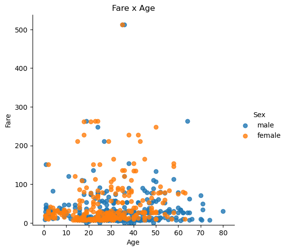
#4.绘制表示乘客票价、年龄、性别的散点图 hue='Sex'根据性别分别用不同颜色表示三点,fit_reg=false 不显示回归线
lm=sns.lmplot(x='Age',y='Fare',data=titantic,hue='Sex',fit_reg=False)
lm.set(title='Fare x Age')
#获取图的坐标轴对象
axes=lm.axes
#设置横轴范围,将下限设为-5
axes[0,0].set_ylim(-5,)
#设置纵轴范围,将下限设为05,上限85
axes[0,0].set_xlim(-5,85)
plt.show()
print('----------4----------')
#5.统计生还人数
print(titantic['Survived'].sum())
print('----------5----------')
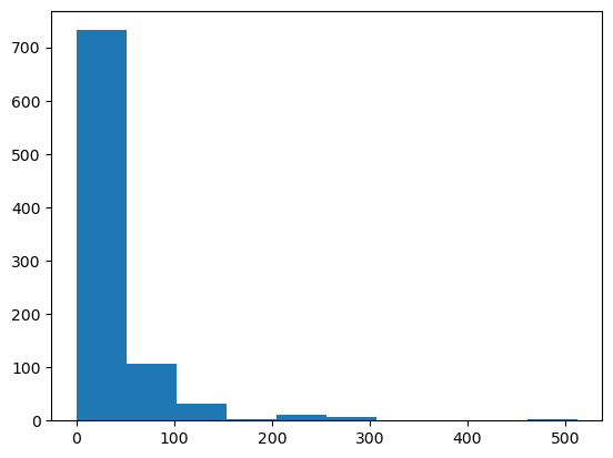
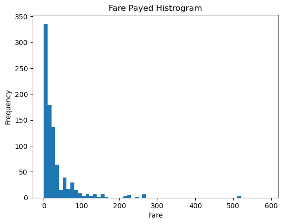
#6. 绘制展示票价的直方图
data=titantic['Fare'].sort_values(ascending=False)
print(data)
binsVal=np.arange(0,600,10)
plt.hist(data,bins=binsVal)
plt.xlabel('Fare')
#纵轴表示价格在某个区间的数据店数量
plt.ylabel('Frequency')
plt.title('Fare Payed Histrogram')
plt.show()
print('----------6----------')
   PassengerId  Survived  Pclass  \
0            1         0       3
1            2         1       1
2            3         1       3
3            4         1       1
4            5         0       3

                                                Name     Sex   Age  SibSp  \
0                            Braund, Mr. Owen Harris    male  22.0      1
1  Cumings, Mrs. John Bradley (Florence Briggs Th...  female  38.0      1
2                             Heikkinen, Miss. Laina  female  26.0      0
3       Futrelle, Mrs. Jacques Heath (Lily May Peel)  female  35.0      1
4                           Allen, Mr. William Henry    male  35.0      0

   Parch            Ticket     Fare Cabin Embarked
0      0         A/5 21171   7.2500   NaN        S
1      0          PC 17599  71.2833   C85        C
2      0  STON/O2. 3101282   7.9250   NaN        S
3      0            113803  53.1000  C123        S
4      0            373450   8.0500   NaN        S
----------1----------
             Survived  Pclass  \
PassengerId
1                   0       3
2                   1       1
3                   1       3
4                   1       1
5                   0       3

                                                          Name     Sex   Age  \
PassengerId
1                                      Braund, Mr. Owen Harris    male  22.0
2            Cumings, Mrs. John Bradley (Florence Briggs Th...  female  38.0
3                                       Heikkinen, Miss. Laina  female  26.0
4                 Futrelle, Mrs. Jacques Heath (Lily May Peel)  female  35.0
5                                     Allen, Mr. William Henry    male  35.0

             SibSp  Parch            Ticket     Fare Cabin Embarked
PassengerId
1                1      0         A/5 21171   7.2500   NaN        S
2                1      0          PC 17599  71.2833   C85        C
3                0      0  STON/O2. 3101282   7.9250   NaN        S
4                1      0            113803  53.1000  C123        S
5                0      0            373450   8.0500   NaN        S
----------2----------
577 314
----------3----------
----------4----------
342
----------5----------
PassengerId
259    512.3292
738    512.3292
680    512.3292
89     263.0000
28     263.0000
         ...
634      0.0000
414      0.0000
823      0.0000
733      0.0000
675      0.0000
Name: Fare, Length: 891, dtype: float64
----------6----------
- 从此看出船票主要集中在0-100的价格区间
8. 创建数据框
#1. 构造数据
raw_data = {"name": ['Bulbasaur', 'Charmander','Squirtle','Caterpie'],
            "evolution": ['Ivysaur','Charmeleon','Wartortle','Metapod'],
            "type": ['grass', 'fire', 'water', 'bug'],
            "hp": [45, 39, 44, 45],
            "pokedex": ['yes', 'no','yes','no']
            }
pokemon = pd.DataFrame(raw_data)
print(pokemon.head())
print('----------1----------')
#2.修改列排序
pokemon=pokemon[['name','type','hp','evolution','pokedex']]
print(pokemon)
print('----------2----------')
#3.新增place列
pokemon['place']=['park','street','lake','forest']
print(pokemon)
print('----------3----------')
#4.查看每列的数据类型
#方法1
print(pokemon.dtypes)
#方法2
print(pokemon.info())
         name   evolution   type  hp pokedex
0   Bulbasaur     Ivysaur  grass  45     yes
1  Charmander  Charmeleon   fire  39      no
2    Squirtle   Wartortle  water  44     yes
3    Caterpie     Metapod    bug  45      no
----------1----------
         name   type  hp   evolution pokedex
0   Bulbasaur  grass  45     Ivysaur     yes
1  Charmander   fire  39  Charmeleon      no
2    Squirtle  water  44   Wartortle     yes
3    Caterpie    bug  45     Metapod      no
----------2----------
         name   type  hp   evolution pokedex   place
0   Bulbasaur  grass  45     Ivysaur     yes    park
1  Charmander   fire  39  Charmeleon      no  street
2    Squirtle  water  44   Wartortle     yes    lake
3    Caterpie    bug  45     Metapod      no  forest
----------3----------
name         object
type         object
hp            int64
evolution    object
pokedex      object
place        object
dtype: object
<class 'pandas.core.frame.DataFrame'>
RangeIndex: 4 entries, 0 to 3
Data columns (total 6 columns):
 #   Column     Non-Null Count  Dtype
---  ------     --------------  -----
 0   name       4 non-null      object
 1   type       4 non-null      object
 2   hp         4 non-null      int64
 3   evolution  4 non-null      object
 4   pokedex    4 non-null      object
 5   place      4 non-null      object
dtypes: int64(1), object(5)
memory usage: 320.0+ bytes
None
9. 时间序列
is_unique 是 Pandas Series 对象的一个属性,用于检查 Series 中的值是否都是唯一的。具体作用如下:
如果 Series 中的所有值都是唯一的,is_unique 返回 True。
如果 Series 中存在重复的值,is_unique 返回 False。
csv_path9="./pandas_data/Apple_stock.csv"
#1:加载数据
apple =pd.read_csv(csv_path9)
print(apple.head())
print('----------1----------')
#2.查看每列的数据类型
print(apple.dtypes)
print('----------2----------')
#3.将Date转换为datetime类型
apple['Date']=pd.to_datetime(apple['Date'])
print(apple['Date'].dtype)
print('----------3----------')
#4.将Date设置为索引
apple.set_index('Date',inplace=True)
print(apple.head())
print('----------4----------')
#5.查看是否有重复日期
print(apple.index.is_unique)
print('----------5----------')
#6. 将index设置为升序
apple.sort_index(ascending=True)
print('----------6----------')
#7.获取每月的最后一个交易日
#注意B表示Business Day为工作日,M为月份
#last() 是采样的聚合函数,它选择每个时间窗口中的最后一个数据点
apple_month = apple.resample('BM').last()
print(apple_month.head())
print('----------7----------')
#8. 计算数据集中最早日期和最晚日期相差多少天
print((apple.index.max()-apple.index.min()).days)
print('----------8----------')
#9. 计算数据集中一共有多少个月
months_count = apple.resample('M').count()
#方法1
print(months_count.shape[0])
#方法2
print(len(months_count))
print('----------9----------')
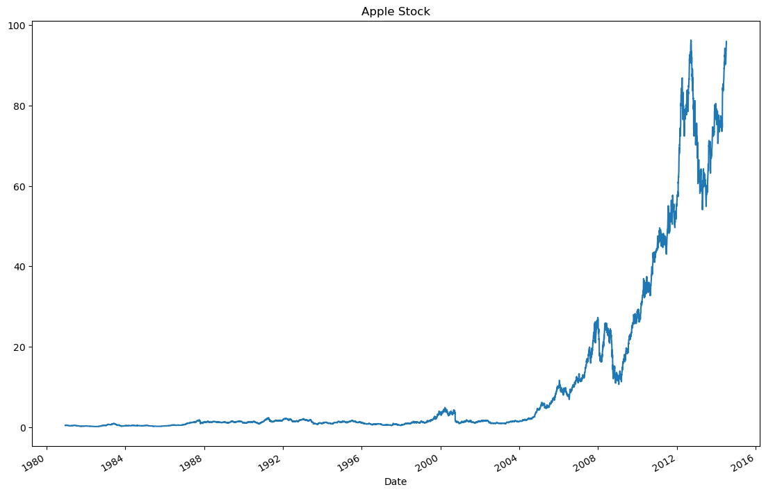
#10. 按照时间顺序可视化Adj Close值【绘制苹果股票的调整后收盘价的折线图】
appl_open = apple['Adj Close'].plot(title = "Apple Stock")
#获取折线图所在的 Figure 对象。
fig = appl_open.get_figure()
fig.set_size_inches(13.5, 9)
plt.show()
         Date   Open   High    Low  Close    Volume  Adj Close
0  2014-07-08  96.27  96.80  93.92  95.35  65130000      95.35
1  2014-07-07  94.14  95.99  94.10  95.97  56305400      95.97
2  2014-07-03  93.67  94.10  93.20  94.03  22891800      94.03
3  2014-07-02  93.87  94.06  93.09  93.48  28420900      93.48
4  2014-07-01  93.52  94.07  93.13  93.52  38170200      93.52
----------1----------
Date          object
Open         float64
High         float64
Low          float64
Close        float64
Volume         int64
Adj Close    float64
dtype: object
----------2----------
datetime64[ns]
----------3----------
             Open   High    Low  Close    Volume  Adj Close
Date
2014-07-08  96.27  96.80  93.92  95.35  65130000      95.35
2014-07-07  94.14  95.99  94.10  95.97  56305400      95.97
2014-07-03  93.67  94.10  93.20  94.03  22891800      94.03
2014-07-02  93.87  94.06  93.09  93.48  28420900      93.48
2014-07-01  93.52  94.07  93.13  93.52  38170200      93.52
----------4----------
True
----------5----------
----------6----------
             Open   High    Low  Close    Volume  Adj Close
Date
1980-12-31  34.25  34.25  34.13  34.13   8937600       0.53
1981-01-30  28.50  28.50  28.25  28.25  11547200       0.44
1981-02-27  26.50  26.75  26.50  26.50   3690400       0.41
1981-03-31  24.75  24.75  24.50  24.50   3998400       0.38
1981-04-30  28.38  28.62  28.38  28.38   3152800       0.44
----------7----------
12261
----------8----------
404
404
----------9----------
10. 删除数据
csv_path10="./pandas_data/iris.csv"
#1:加载数据
iris =pd.read_csv(csv_path10)
print(iris.head())
print('----------1----------')
#2.添加列名称
iris = pd.read_csv(csv_path10, names=['sepal_length', 'sepal_width', 'petal_length', 'petal_width', 'class'])
print(iris.head())

print('----------2----------')
#3.查看是否有缺失值
print(iris.isnull().sum())

print('----------3----------')
#4.将列petal_length的第10到19行设置为缺失值
iris.iloc[10:20,2:3]=np.nan
print(iris.head(20))
print('----------4----------')
#5.将缺失值替换为1.0
iris['petal_length'].fillna(1,inplace=True)
print(iris.head(20))
print('----------5----------')
#6.删除class列
#方法1
iris.drop('class',axis=1,inplace=True)
print(iris.head())
#方法2
# del iris['class']
# print(iris.head())
print('----------6----------')
#7.数据集前三行设置为NaN
iris.iloc[0:3,:]=np.nan
print(iris.head())

print('----------7----------')
#8. 删除含有NaN的行
iris=iris.dropna(how='any')
print('----------8----------')
#9. 重置索引
iris.reset_index(drop=True)
print(iris.head())
print('----------9----------')
   5.1  3.5  1.4  0.2  Iris-setosa
0  4.9  3.0  1.4  0.2  Iris-setosa
1  4.7  3.2  1.3  0.2  Iris-setosa
2  4.6  3.1  1.5  0.2  Iris-setosa
3  5.0  3.6  1.4  0.2  Iris-setosa
4  5.4  3.9  1.7  0.4  Iris-setosa
----------1----------
   sepal_length  sepal_width  petal_length  petal_width        class
0           5.1          3.5           1.4          0.2  Iris-setosa
1           4.9          3.0           1.4          0.2  Iris-setosa
2           4.7          3.2           1.3          0.2  Iris-setosa
3           4.6          3.1           1.5          0.2  Iris-setosa
4           5.0          3.6           1.4          0.2  Iris-setosa
----------2----------
sepal_length    0
sepal_width     0
petal_length    0
petal_width     0
class           0
dtype: int64
----------3----------
    sepal_length  sepal_width  petal_length  petal_width        class
0            5.1          3.5           1.4          0.2  Iris-setosa
1            4.9          3.0           1.4          0.2  Iris-setosa
2            4.7          3.2           1.3          0.2  Iris-setosa
3            4.6          3.1           1.5          0.2  Iris-setosa
4            5.0          3.6           1.4          0.2  Iris-setosa
5            5.4          3.9           1.7          0.4  Iris-setosa
6            4.6          3.4           1.4          0.3  Iris-setosa
7            5.0          3.4           1.5          0.2  Iris-setosa
8            4.4          2.9           1.4          0.2  Iris-setosa
9            4.9          3.1           1.5          0.1  Iris-setosa
10           5.4          3.7           NaN          0.2  Iris-setosa
11           4.8          3.4           NaN          0.2  Iris-setosa
12           4.8          3.0           NaN          0.1  Iris-setosa
13           4.3          3.0           NaN          0.1  Iris-setosa
14           5.8          4.0           NaN          0.2  Iris-setosa
15           5.7          4.4           NaN          0.4  Iris-setosa
16           5.4          3.9           NaN          0.4  Iris-setosa
17           5.1          3.5           NaN          0.3  Iris-setosa
18           5.7          3.8           NaN          0.3  Iris-setosa
19           5.1          3.8           NaN          0.3  Iris-setosa
----------4----------
    sepal_length  sepal_width  petal_length  petal_width        class
0            5.1          3.5           1.4          0.2  Iris-setosa
1            4.9          3.0           1.4          0.2  Iris-setosa
2            4.7          3.2           1.3          0.2  Iris-setosa
3            4.6          3.1           1.5          0.2  Iris-setosa
4            5.0          3.6           1.4          0.2  Iris-setosa
5            5.4          3.9           1.7          0.4  Iris-setosa
6            4.6          3.4           1.4          0.3  Iris-setosa
7            5.0          3.4           1.5          0.2  Iris-setosa
8            4.4          2.9           1.4          0.2  Iris-setosa
9            4.9          3.1           1.5          0.1  Iris-setosa
10           5.4          3.7           1.0          0.2  Iris-setosa
11           4.8          3.4           1.0          0.2  Iris-setosa
12           4.8          3.0           1.0          0.1  Iris-setosa
13           4.3          3.0           1.0          0.1  Iris-setosa
14           5.8          4.0           1.0          0.2  Iris-setosa
15           5.7          4.4           1.0          0.4  Iris-setosa
16           5.4          3.9           1.0          0.4  Iris-setosa
17           5.1          3.5           1.0          0.3  Iris-setosa
18           5.7          3.8           1.0          0.3  Iris-setosa
19           5.1          3.8           1.0          0.3  Iris-setosa
----------5----------
   sepal_length  sepal_width  petal_length  petal_width
0           5.1          3.5           1.4          0.2
1           4.9          3.0           1.4          0.2
2           4.7          3.2           1.3          0.2
3           4.6          3.1           1.5          0.2
4           5.0          3.6           1.4          0.2
----------6----------
   sepal_length  sepal_width  petal_length  petal_width
0           NaN          NaN           NaN          NaN
1           NaN          NaN           NaN          NaN
2           NaN          NaN           NaN          NaN
3           4.6          3.1           1.5          0.2
4           5.0          3.6           1.4          0.2
----------7----------
----------8----------
   sepal_length  sepal_width  petal_length  petal_width
3           4.6          3.1           1.5          0.2
4           5.0          3.6           1.4          0.2
5           5.4          3.9           1.7          0.4
6           4.6          3.4           1.4          0.3
7           5.0          3.4           1.5          0.2
----------9----------