目录
介绍:
二、数据
2.1引用数据
2.2检查缺失数据
2.2.1手动检查缺失数据
2.2.2查看某一个特征值为空数据
2.3补充缺失数据
2.3.1盒图
2.3.2手动用均值填补缺失数据
2.3.3手动用类别填补缺失数据
三、数据分析
3.1男女生存比例
3.2男女生存数
3.3船舱级别生存比例
3.4船舱生存与死亡比例
3.5票价与生存关系
3.6年龄与生存关系
3.7性别年龄与生存关系
3.8性别、登口岸、年龄与生存关系
3.9性别、票价、年龄与生存关系
四、数据处理
4.1处理性别
4.2热图表相关性
4.3姓名处理
4.4处理家庭大小
4.5清除票
4.5处理票价
4.6数据整理
4.7用RandomForestRegressor预测年龄填补缺失数据
五、建模
5.1LogisticRegression建模
5.2Decision Tree建模
5.3randomforest建模
5.4Adaboost建模
介绍:
AdaBoost(Adaptive Boosting)是一种集成学习方法,用于提高机器学习算法的准确性。它通过训练一系列弱分类器(即准确率略高于随机猜测的分类器),然后将它们组合成一个强分类器。
AdaBoost的基本思想是对训练样本进行加权,将分类错误的样本权值增大,再训练下一个分类器。经过多轮迭代,每个样本都会得到不同的权值,并且每个分类器都有一定的权重。最终,AdaBoost通过对所有分类器的加权求和,得到最终的分类结果。
在AdaBoost中,每个弱分类器的训练过程如下:
- 初始化样本权值为相等值。
- 使用权值训练一个弱分类器。
- 根据分类错误率计算该分类器的权重。
- 更新样本权值,增加分类错误的样本权值,并减小分类正确的样本权值。
- 重复步骤2到4,直到达到指定的弱分类器个数或达到某个条件。
最终的强分类器是将每个弱分类器的输出加权求和,并根据总体输出判断样本的分类。
AdaBoost模型有一些特点:
- 适用于二分类和多分类问题。
- 对于弱分类器的选择没有严格的限制,可以使用任何分类器作为基分类器。
- 在训练过程中,每个样本都被赋予不同的权重,以便更加关注错误分类的样本。
- 可以减少过拟合问题,因为它将注意力集中在难以分类的样本上。
- AdaBoost的训练速度较快,预测速度也较快。
总的来说,AdaBoost是一种强大的集成学习算法,可以通过组合多个弱分类器来提高分类的准确性。它在实际应用中取得了很好的效果,并广泛应用于各个领域。
二、数据
2.1引用数据
import pandas as pd
import numpy as np
import matplotlib.pyplot as plt
import seaborn as sns
%matplotlib inline

import warnings
warnings.filterwarnings('ignore')##忽略警告

train = pd.read_csv("train.csv")
test = pd.read_csv("test.csv")

passengerid = test.PassengerId

print(train.info())
print('*'*80)
print(test.info())
'''结果:
<class 'pandas.core.frame.DataFrame'>
RangeIndex: 891 entries, 0 to 890
Data columns (total 12 columns):
 #   Column       Non-Null Count  Dtype
---  ------       --------------  -----
 0   PassengerId  891 non-null    int64
 1   Survived     891 non-null    int64
 2   Pclass       891 non-null    int64
 3   Name         891 non-null    object
 4   Sex          891 non-null    object
 5   Age          714 non-null    float64
 6   SibSp        891 non-null    int64
 7   Parch        891 non-null    int64
 8   Ticket       891 non-null    object
 9   Fare         891 non-null    float64
 10  Cabin        204 non-null    object
 11  Embarked     889 non-null    object
dtypes: float64(2), int64(5), object(5)
memory usage: 83.7+ KB
None
********************************************************************************
<class 'pandas.core.frame.DataFrame'>
RangeIndex: 418 entries, 0 to 417
Data columns (total 12 columns):
 #   Column       Non-Null Count  Dtype
---  ------       --------------  -----
 0   PassengerId  418 non-null    int64
 1   Survived     418 non-null    int64
 2   Pclass       418 non-null    int64
 3   Name         418 non-null    object
 4   Sex          418 non-null    object
 5   Age          332 non-null    float64
 6   SibSp        418 non-null    int64
 7   Parch        418 non-null    int64
 8   Ticket       418 non-null    object
 9   Fare         417 non-null    float64
 10  Cabin        91 non-null     object
 11  Embarked     418 non-null    object
dtypes: float64(2), int64(5), object(5)
memory usage: 39.3+ KB
None
'''
2.2检查缺失数据
2.2.1手动检查缺失数据
def missing_percentage(df):#显示空缺数据
    total = df.isnull().sum().sort_values(ascending=False)
    percent = round(df.isnull().sum().sort_values(ascending=False)/len(df)*100,2)
    return pd.concat([total,percent],axis=1,keys=['Total','Percent'])

missing_percentage(train)#检查缺失数据
'''结果:
 	Total 	Percent
Cabin 	687 	77.10
Age 	177 	19.87
Embarked 	2 	0.22
PassengerId 	0 	0.00
Survived 	0 	0.00
Pclass 	0 	0.00
Name 	0 	0.00
Sex 	0 	0.00
SibSp 	0 	0.00
Parch 	0 	0.00
Ticket 	0 	0.00
Fare 	0 	0.00
'''

missing_percentage(test)
'''结果:
 	Total 	Percent
Cabin 	327 	78.23
Age 	86 	20.57
Fare 	1 	0.24
PassengerId 	0 	0.00
Survived 	0 	0.00
Pclass 	0 	0.00
Name 	0 	0.00
Sex 	0 	0.00
SibSp 	0 	0.00
Parch 	0 	0.00
Ticket 	0 	0.00
Embarked 	0 	0.00
'''
def percent_value_counts(df,feature):#统计一个特征值的特征类别
percent = pd.DataFrame(round(df.loc[:,feature].value_counts(dropna=False,normalize=True)*100,2))
total = pd.DataFrame(df.loc[:,feature].value_counts(dropna=False))
total.columns=["Total"]
percent.columns=['Percent']
return pd.concat([total,percent],axis=1)
percent_value_counts(train,'Embarked')
'''结果:
Total Percent
S 644 72.28
C 168 18.86
Q 77 8.64
NaN 2 0.22
'''2.2.2查看某一个特征值为空数据
train[train.Embarked.isnull()]#查看某一特征值为空的数据
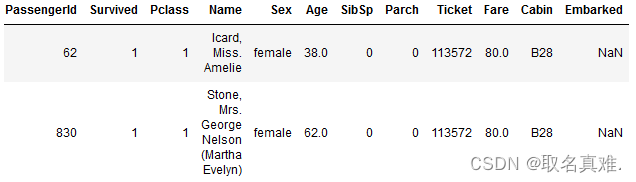
2.3补充缺失数据
2.3.1盒图
sns.set_style('darkgrid')
fig, ax = plt.subplots(figsize=(16,12),ncols=2)#前面表示图的大小,后面表示两个图

ax1 = sns.boxplot(x="Embarked", y="Fare", hue="Pclass", data=train, ax = ax[0]);
ax2 = sns.boxplot(x="Embarked", y="Fare", hue="Pclass", data=test,ax = ax[1]);

ax1.set_title("Training set", fontsize=18)
ax2.set_title('Test set', fontsize=18)

## Fixing Legends
leg_1 = ax1.get_legend()
leg_1.set_title("PClass")
legs = leg_1.texts
legs[0].set_text('upper')
legs[1].set_text('Middle')
legs[2].set_text('Lower')

fig.show( )#可以看均值,通过均值补充空的值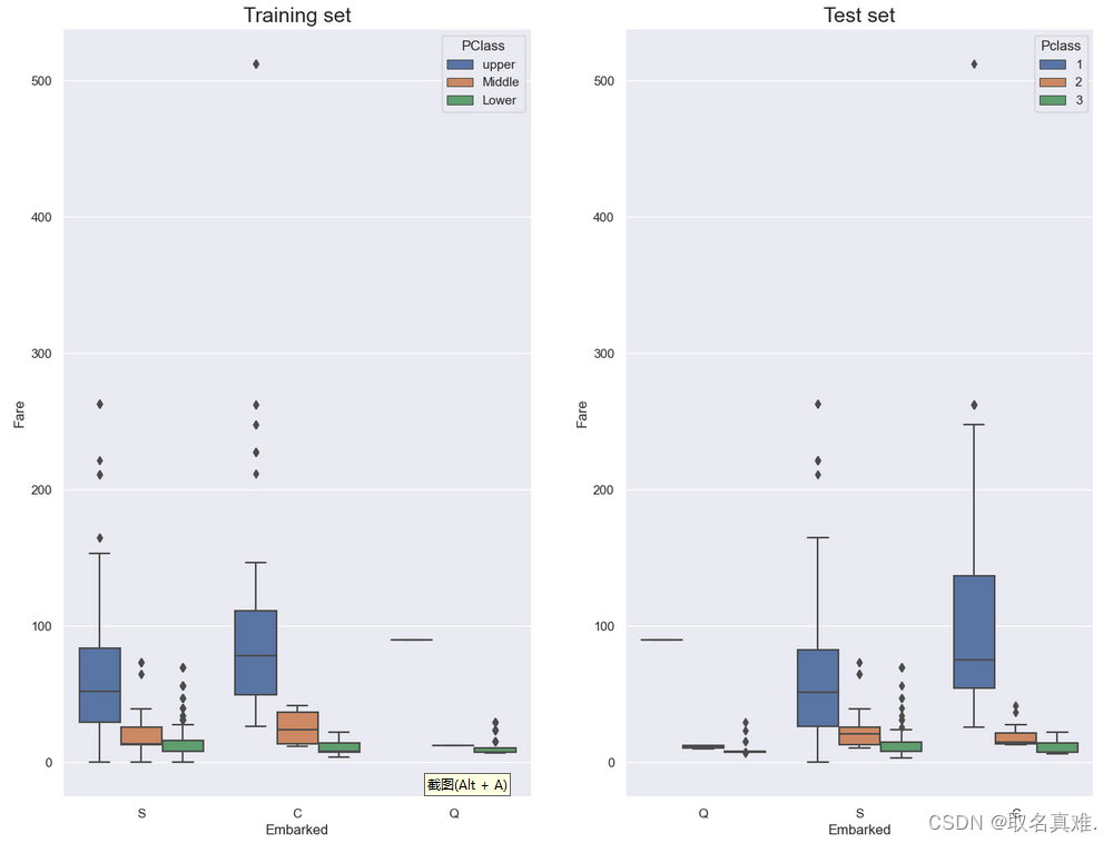
train.Embarked.fillna("C",inplace=True)#填充空数据

##缺失数据的Pclass为1,票价为80,根据盒图可以看出Pclass为1,票价均值为80的c
#所以用c补充数据
2.3.2手动用均值填补缺失数据
print("Train Cabin missing:" + str(train.Cabin.isnull().sum()/len(train.Cabin)))
#结果:Train Cabin missing:0.7710437710437711

'''缺失数据量大,把训练集和测试集合并'''
survivers = train.Survived
train.drop(["Survived"],axis=1, inplace=True)

all_data = pd.concat([train,test],ignore_index=False)#train和test连接起来

#* Assign all the null values to N
all_data.Cabin.fillna("N", inplace=True)#先用N补充空数据


percent_value_counts(all_data,"Cabin")#统计一个特征值的特征个数
'''结果:
 	Total 	Percent
N 	1014 	77.46
C 	94 	    7.18
B 	65 	    4.97
D 	46 	    3.51
E 	41 	    3.13
A 	22 	    1.68
F 	21 	    1.60
G 	5 	    0.38
T 	1 	    0.08
'''

all_data.groupby("Cabin")['Fare'].mean().sort_values()#每个舱位的票价均值
'''结果:
Cabin
G     14.205000
F     18.079367
N     19.132707
T     35.500000
A     41.244314
D     53.007339
E     54.564634
C    107.926598
B    122.383078
Name: Fare, dtype: float64
'''
def cabin_estimator(i):#"""grouping cabin feature by the first letter"""
a = 0
if i<16:
a="G"
elif i>=16 and i<27:
a="F"
elif i>=27 and i<38:
a="T"
elif i>=38 and i<47:
a="A"
elif i>= 47 and i<53:
a="E"
elif i>= 53 and i<54:
a="D"
elif i>=54 and i<116:
a='C'
else:
a="B"
return a
#把为N的挑出来,不为N挑出来
with_N = all_data[all_data.Cabin == "N"]
without_N = all_data[all_data.Cabin != "N"]
##opplying cabin estimator function.
with_N['Cabin'] = with_N.Fare.apply(lambda x: cabin_estimator(x))#根据票价赋值
## getting back train.
all_data = pd.concat([with_N, without_N],axis=0)#连接在一起
## PassengerId helps us separate train and test.
all_data.sort_values(by ='PassengerId', inplace=True)
## Separating train and test from all_data.
train = all_data[:891]#再分训练集和测试集
test = all_data[891:]
#adding saved target variable with train.
train['Survived']=survivers2.3.3手动用类别填补缺失数据
test[test.Fare.isnull()]
'''结果:
 	PassengerId 	Pclass 	Name 	Sex 	Age 	SibSp 	Parch 	Ticket 	Fare 	Cabin 	Embarked 	Survived
152 	1044 	3 	Storey, Mr. Thomas 	male 	60.5 	0 	0 	3701 	NaN 	B 	S 	0.0
'''

missing_value = test[(test.Pclass == 3)&
                     (test.Embarked == 'S')&
                     (test.Sex == 'male')].Fare.mean()#求这类乘客的票价均值

test.Fare.fillna(missing_value,inplace=True)#将均值赋给空
三、数据分析
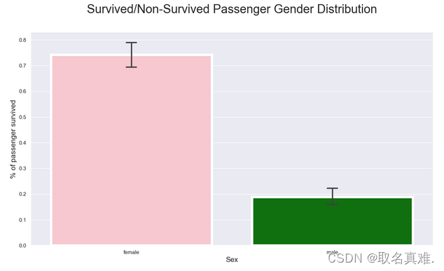
3.1男女生存比例
import seaborn as sns
pal = {'male':"green", 'female':"Pink"}
sns.set(style="darkgrid")
plt.subplots(figsize = (15,8))
ax = sns.barplot(x = "Sex",
                 y = "Survived",
                 data=train,
                 palette = pal,
                 linewidth=5,
                 order = ['female','male'],
                 capsize = .05,

                )

plt.title("Survived/Non-Survived Passenger Gender Distribution", fontsize = 25,loc = 'center', pad = 40)
plt.ylabel("% of passenger survived", fontsize = 15, )
plt.xlabel("Sex",fontsize = 15);
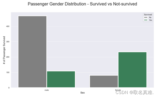
3.2男女生存数
pal = {1:"seagreen", 0:"gray"}
sns.set(style="darkgrid")
plt.subplots(figsize = (15,8))
ax = sns.countplot(x = "Sex",
                   hue="Survived",
                   data = train,
                   linewidth=4,
                   palette = pal
)

## Fixing title, xlabel and ylabel
plt.title("Passenger Gender Distribution - Survived vs Not-survived", fontsize = 25, pad=40)
plt.xlabel("Sex", fontsize = 15);
plt.ylabel("# of Passenger Survived", fontsize = 15)

## Fixing xticks
#labels = ['Female', 'Male']
#plt.xticks(sorted(train.Sex.unique()), labels)

## Fixing legends
leg = ax.get_legend()
leg.set_title("Survived")
legs = leg.texts
legs[0].set_text("No")
legs[1].set_text("Yes")
plt.show()
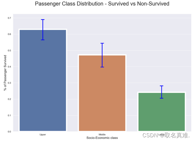
3.3船舱级别生存比例
plt.subplots(figsize = (15,10))
sns.barplot(x = "Pclass",
            y = "Survived",
            data=train,
            linewidth=6,
            capsize = .05,
            errcolor='blue',
            errwidth = 3


           )
plt.title("Passenger Class Distribution - Survived vs Non-Survived", fontsize = 25, pad=40)
plt.xlabel("Socio-Economic class", fontsize = 15);
plt.ylabel("% of Passenger Survived", fontsize = 15);
names = ['Upper', 'Middle', 'Lower']
#val = sorted(train.Pclass.unique())
val = [0,1,2] ## this is just a temporary trick to get the label right.
plt.xticks(val, names);
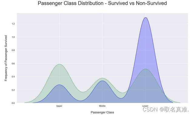
3.4船舱生存与死亡比例
# Kernel Density Plot
fig = plt.figure(figsize=(15,8),)
## I have included to different ways to code a plot below, choose the one that suites you.
ax=sns.kdeplot(train.Pclass[train.Survived == 0] ,
               color='blue',
               shade=True,
               label='not survived')
ax=sns.kdeplot(train.loc[(train['Survived'] == 1),'Pclass'] ,
               color='g',
               shade=True,
               label='survived',
              )
plt.title('Passenger Class Distribution - Survived vs Non-Survived', fontsize = 25, pad = 40)
plt.ylabel("Frequency of Passenger Survived", fontsize = 15, labelpad = 20)
plt.xlabel("Passenger Class", fontsize = 15,labelpad =20)
## Converting xticks into words for better understanding
labels = ['Upper', 'Middle', 'Lower']
plt.xticks(sorted(train.Pclass.unique()), labels);
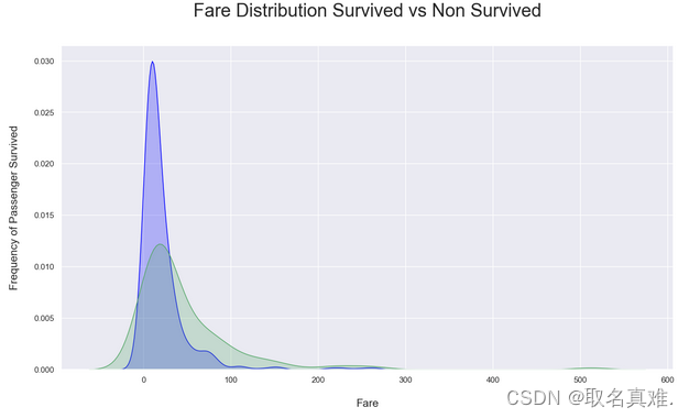
3.5票价与生存关系
# Kernel Density Plot
fig = plt.figure(figsize=(15,8),)
ax=sns.kdeplot(train.loc[(train['Survived'] == 0),'Fare'] , color='blue',shade=True,label='not survived')
ax=sns.kdeplot(train.loc[(train['Survived'] == 1),'Fare'] , color='g',shade=True, label='survived')
plt.title('Fare Distribution Survived vs Non Survived', fontsize = 25, pad = 40)
plt.ylabel("Frequency of Passenger Survived", fontsize = 15, labelpad = 20)
plt.xlabel("Fare", fontsize = 15, labelpad = 20);
3.6年龄与生存关系
# Kernel Density Plot
fig = plt.figure(figsize=(15,8),)
ax=sns.kdeplot(train.loc[(train['Survived'] == 0),'Age'] , color='blue',shade=True,label='not survived')
ax=sns.kdeplot(train.loc[(train['Survived'] == 1),'Age'] , color='g',shade=True, label='survived')
plt.title('Age Distribution - Surviver V.S. Non Survivors', fontsize = 25, pad = 40)
plt.xlabel("Age", fontsize = 15, labelpad = 20)
plt.ylabel('Frequency', fontsize = 15, labelpad= 20); 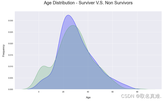
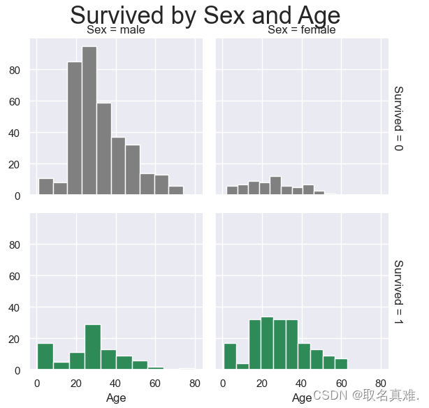
3.7性别年龄与生存关系
pal = {1:"seagreen", 0:"gray"}
g = sns.FacetGrid(train,  col="Sex", row="Survived", margin_titles=True, hue = "Survived",
                  palette=pal)
g = g.map(plt.hist, "Age", edgecolor = 'white');
g.fig.suptitle("Survived by Sex and Age", size = 25)
plt.subplots_adjust(top=0.90)
3.8性别、登口岸、年龄与生存关系
g = sns.FacetGrid(train, col="Sex", row="Embarked", margin_titles=True, hue = "Survived",
                  palette = pal
                  )
g = g.map(plt.hist, "Age", edgecolor = 'white').add_legend();
g.fig.suptitle("Survived by Sex and Age", size = 25)
plt.subplots_adjust(top=0.90)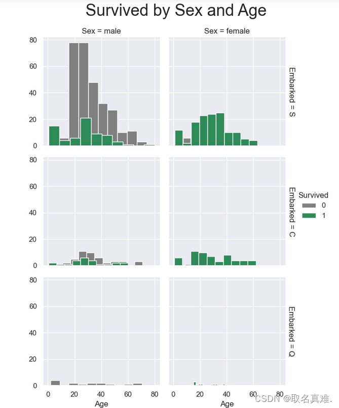
3.9性别、票价、年龄与生存关系
g = sns.FacetGrid(train,hue="Survived", col ="Sex", margin_titles=True,
                palette=pal,)
g.map(plt.scatter, "Fare", "Age",edgecolor="w").add_legend()
g.fig.suptitle("Survived by Sex, Fare and Age", size = 25)
plt.subplots_adjust(top=0.85) 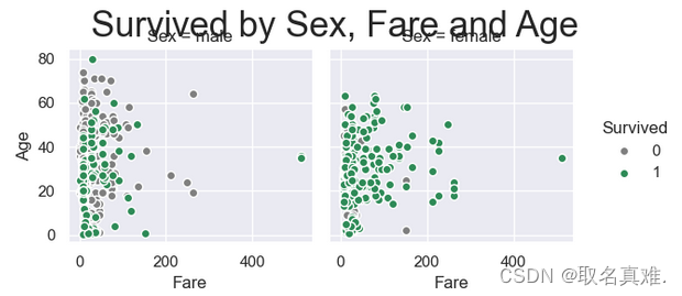
四、数据处理
4.1处理性别
male_mean = train[train['Sex'] == 1].Survived.mean()

female_mean = train[train['Sex'] == 0].Survived.mean()
print ("Male survival mean: " + str(male_mean))
print ("female survival mean: " + str(female_mean))

print ("The mean difference between male and female survival rate: " + str(female_mean - male_mean))

'''结果:
Male survival mean: 0.18890814558058924
female survival mean: 0.7420382165605095
The mean difference between male and female survival rate: 0.5531300709799203
'''

# separating male and female dataframe.
import random
male = train[train['Sex'] == 1]
female = train[train['Sex'] == 0]

## empty list for storing mean sample
m_mean_samples = []
f_mean_samples = []

for i in range(50):
    m_mean_samples.append(np.mean(random.sample(list(male['Survived']),50,)))
    f_mean_samples.append(np.mean(random.sample(list(female['Survived']),50,)))


# Print them out
print (f"Male mean sample mean: {round(np.mean(m_mean_samples),2)}")
print (f"Female mean sample mean: {round(np.mean(f_mean_samples),2)}")
print (f"Difference between male and female mean sample mean: {round(np.mean(f_mean_samples) - np.mean(m_mean_samples),2)}")


'''结果:
Male mean sample mean: 0.18
Female mean sample mean: 0.74
Difference between male and female mean sample mean: 0.56
'''
# Placing 0 for female and
# 1 for male in the "Sex" column.
train['Sex'] = train.Sex.apply(lambda x: 0 if x == "female" else 1)
test['Sex'] = test.Sex.apply(lambda x: 0 if x == "female" else 1)train.describe()#数据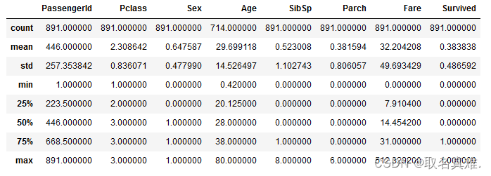
survived_summary = train.groupby("Survived")
survived_summary.mean().reset_index()
'''结果:
 	Survived 	PassengerId 	Pclass 	Sex 	Age 	SibSp 	Parch 	Fare
0 	0 	447.016393 	2.531876 	0.852459 	30.626179 	0.553734 	0.329690 	22.117887
1 	1 	444.368421 	1.950292 	0.318713 	28.343690 	0.473684 	0.464912 	48.395408
'''

survived_summary = train.groupby("Sex")
survived_summary.mean().reset_index()
'''结果:
 	Sex 	PassengerId 	Pclass 	Age 	SibSp 	Parch 	Fare 	Survived
0 	0 	431.028662 	2.159236 	27.915709 	0.694268 	0.649682 	44.479818 	0.742038
1 	1 	454.147314 	2.389948 	30.726645 	0.429809 	0.235702 	25.523893 	0.188908
'''

survived_summary = train.groupby("Pclass")
survived_summary.mean().reset_index()
'''结果:
 	Pclass 	PassengerId 	Sex 	Age 	SibSp 	Parch 	Fare 	Survived
0 	1 	461.597222 	0.564815 	38.233441 	0.416667 	0.356481 	84.154687 	0.629630
1 	2 	445.956522 	0.586957 	29.877630 	0.402174 	0.380435 	20.662183 	0.472826
2 	3 	439.154786 	0.706721 	25.140620 	0.615071 	0.393075 	13.675550 	0.242363
'''

pd.DataFrame(abs(train.corr()["Survived"]).sort_values(ascending=False))#相关性
'''结果:

 	Survived
Survived 	1.000000
Sex 	0.543351
Pclass 	0.338481
Fare 	0.257307
Parch 	0.081629
Age 	0.077221
SibSp 	0.035322
PassengerId 	0.005007
'''
4.2热图表相关性
corr = train.corr()**2
corr.Survived.sort_values(ascending = False)


## heatmeap to see the correlatton between features
# Generate a mask for the upper triangle (taken from seaborn example gallery)
import numpy as np
mask = np.zeros_like(train.corr(),dtype=bool)
mask[np.triu_indices_from(mask)]  = True
sns.set_style("whitegrid")

plt.subplots(figsize = (15,12))
sns.heatmap(train.corr(),
            annot=True,
            mask = mask,
            cmap = 'RdBu', ## in order to reverse the bar replace "RdBu" with "RdBur'
            linewidths=.9,
            linecolor="white",
             fmt='.2g',
            center = 0,
            square=True)
plt.title("correlations Among Features", y = 1.03,fontsize = 20, pad = 40);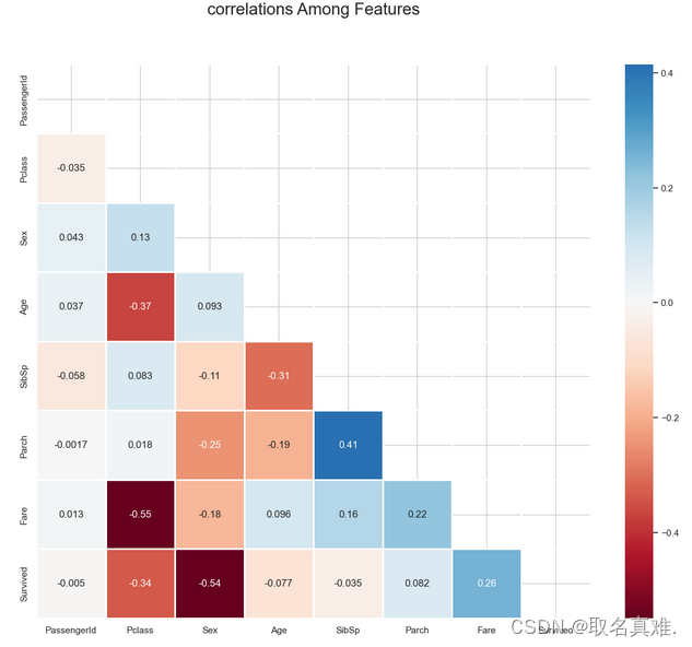
4.3姓名处理
# Creating a new colomn with a
train['name_length'] = [len(i) for i in train.Name]
test['name_length'] = [len(i) for i in test.Name]

def name_length_group(size):
    a = ''
    if (size <=20):
        a = 'short'
    elif (size <=35):
        a = 'medium'
    elif (size <=45):
        a = 'good'
    else:
        a = 'long'
    return a


train['nLength_group'] = train['name_length'].map(name_length_group)
test['nLength_group'] = test['name_length'].map(name_length_group)

## Here "map" is python's built-in function.
## "map" function basically takes a function and
## returns an iterable list/tuple or in this case series.
## However,"map" can also be used like map(function) e.g. map(name_length_group)
## or map(function, iterable{list, tuple}) e.g. map(name_length_group, train[feature]]).
## However, here we don't need to use parameter("size") for name_length_group because when we
## used the map function like ".map" with a series before dot, we are basically hinting that series
## and the iterable. This is similar to .append approach in python. list.append(a) meaning applying append on list.


## cuts the column by given bins based on the range of name_length
#group_names = ['short', 'medium', 'good', 'long']
#train['name_len_group'] = pd.cut(train['name_length'], bins = 4, labels=group_names)
## get the title from the name
train["title"] = [i.split('.')[0] for i in train.Name]
train["title"] = [i.split(',')[1] for i in train.title]
## Whenever we split like that, there is a good change that
#we will end up with white space around our string values. Let's check that.
print(train.title.unique())
'''结果:
[' Mr' ' Mrs' ' Miss' ' Master' ' Don' ' Rev' ' Dr' ' Mme' ' Ms' ' Major'
' Lady' ' Sir' ' Mlle' ' Col' ' Capt' ' the Countess' ' Jonkheer']
'''
## Let's fix that
train.title = train.title.apply(lambda x: x.strip())
## We can also combile all three lines above for test set here
test['title'] = [i.split('.')[0].split(',')[1].strip() for i in test.Name]
## However it is important to be able to write readable code, and the line above is not so readable.
## Let's replace some of the rare values with the keyword 'rare' and other word choice of our own.
## train Data
train["title"] = [i.replace('Ms', 'Miss') for i in train.title]
train["title"] = [i.replace('Mlle', 'Miss') for i in train.title]
train["title"] = [i.replace('Mme', 'Mrs') for i in train.title]
train["title"] = [i.replace('Dr', 'rare') for i in train.title]
train["title"] = [i.replace('Col', 'rare') for i in train.title]
train["title"] = [i.replace('Major', 'rare') for i in train.title]
train["title"] = [i.replace('Don', 'rare') for i in train.title]
train["title"] = [i.replace('Jonkheer', 'rare') for i in train.title]
train["title"] = [i.replace('Sir', 'rare') for i in train.title]
train["title"] = [i.replace('Lady', 'rare') for i in train.title]
train["title"] = [i.replace('Capt', 'rare') for i in train.title]
train["title"] = [i.replace('the Countess', 'rare') for i in train.title]
train["title"] = [i.replace('Rev', 'rare') for i in train.title]
## Now in programming there is a term called DRY(Don't repeat yourself), whenever we are repeating
## same code over and over again, there should be a light-bulb turning on in our head and make us think
## to code in a way that is not repeating or dull. Let's write a function to do exactly what we
## did in the code above, only not repeating and more interesting.
## we are writing a function that can help us modify title column
def fuse_title(feature):
"""
This function helps modifying the title column
"""
result = ''
if feature in ['the Countess','Capt','Lady','Sir','Jonkheer','Don','Major','Col', 'Rev', 'Dona', 'Dr']:
result = 'rare'
elif feature in ['Ms', 'Mlle']:
result = 'Miss'
elif feature == 'Mme':
result = 'Mrs'
else:
result = feature
return result
test.title = test.title.map(fuse_title)
train.title = train.title.map(fuse_title)
4.4处理家庭大小
## bin the family size.
def family_group(size):
    """
    This funciton groups(loner, small, large) family based on family size
    """

    a = ''
    if (size <= 1):
        a = 'loner'
    elif (size <= 4):
        a = 'small'
    else:
        a = 'large'
    return a

## apply the family_group function in family_size
train['family_group'] = train['family_size'].map(family_group)
test['family_group'] = test['family_size'].map(family_group)

train['is_alone'] = [1 if i<2 else 0 for i in train.family_size]
test['is_alone'] = [1 if i<2 else 0 for i in test.family_size]
4.5清除票
train.drop(['Ticket'],axis=1,inplace=True)
test.drop(['Ticket'],axis=1,inplace=True)
4.5处理票价
## Calculating fare based on family size.
train['calculated_fare'] = train.Fare/train.family_size
test['calculated_fare'] = test.Fare/test.family_size


def fare_group(fare):
    """
    This function creates a fare group based on the fare provided
    """

    a= ''
    if fare <= 4:
        a = 'Very_low'
    elif fare <= 10:
        a = 'low'
    elif fare <= 20:
        a = 'mid'
    elif fare <= 45:
        a = 'high'
    else:
        a = "very_high"
    return a

train['fare_group'] = train['calculated_fare'].map(fare_group)
test['fare_group'] = test['calculated_fare'].map(fare_group)

#train['fare_group'] = pd.cut(train['calculated_fare'], bins = 4, labels=groups)
4.6数据整理
train.drop(['PassengerId'], axis=1, inplace=True)

test.drop(['PassengerId'], axis=1, inplace=True)


train = pd.get_dummies(train, columns=['title',"Pclass", 'Cabin','Embarked','nLength_group', 'family_group', 'fare_group'], drop_first=False)
test = pd.get_dummies(test, columns=['title',"Pclass",'Cabin','Embarked','nLength_group', 'family_group', 'fare_group'], drop_first=False)
train.drop(['family_size','Name', 'Fare','name_length'], axis=1, inplace=True)
test.drop(['Name','family_size',"Fare",'name_length'], axis=1, inplace=True)


## rearranging the columns so that I can easily use the dataframe to predict the missing age values.
train = pd.concat([train[["Survived", "Age", "Sex","SibSp","Parch"]], train.loc[:,"is_alone":]], axis=1)
test = pd.concat([test[["Age", "Sex"]], test.loc[:,"SibSp":]], axis=1)

train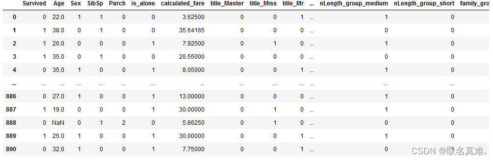
4.7用RandomForestRegressor预测年龄填补缺失数据
#用RandomForestRegressor预测年龄
# Importing RandomForestRegressor
from sklearn.ensemble import RandomForestRegressor

## writing a function that takes a dataframe with missing values and outputs it by filling the missing values.
def completing_age(df):
    ## gettting all the features except survived
    age_df = df.loc[:,"Age":]

    temp_train = age_df.loc[age_df.Age.notnull()] ## df with age values
    temp_test = age_df.loc[age_df.Age.isnull()] ## df without age values

    y = temp_train.Age.values ## setting target variables(age) in y
    x = temp_train.loc[:, "Sex":].values

    rfr = RandomForestRegressor(n_estimators=1500, n_jobs=-1)
    rfr.fit(x, y)

    predicted_age = rfr.predict(temp_test.loc[:, "Sex":])

    df.loc[df.Age.isnull(), "Age"] = predicted_age


    return df

## Implementing the completing_age function in both train and test dataset.
completing_age(train)
completing_age(test);

## Let's look at the his
plt.subplots(figsize = (22,10),)
sns.distplot(train.Age, bins = 100, kde = True, rug = False, norm_hist=False);
## create bins for age
def age_group_fun(age):
    """
    This function creates a bin for age
    """
    a = ''
    if age <= 1:
        a = 'infant'
    elif age <= 4:
        a = 'toddler'
    elif age <= 13:
        a = 'child'
    elif age <= 18:
        a = 'teenager'
    elif age <= 35:
        a = 'Young_Adult'
    elif age <= 45:
        a = 'adult'
    elif age <= 55:
        a = 'middle_aged'
    elif age <= 65:
        a = 'senior_citizen'
    else:
        a = 'old'
    return a

## Applying "age_group_fun" function to the "Age" column.
train['age_group'] = train['Age'].map(age_group_fun)
test['age_group'] = test['Age'].map(age_group_fun)

## Creating dummies for "age_group" feature.
train = pd.get_dummies(train,columns=['age_group'], drop_first=True)
test = pd.get_dummies(test,columns=['age_group'], drop_first=True);
五、建模
# separating our independent and dependent variable
X = train.drop(['Survived'], axis = 1)
y = train["Survived"]

from sklearn.model_selection import train_test_split
X_train, X_test, y_train, y_test = train_test_split(X, y,test_size = .33, random_state=0)

# Feature Scaling 数据差异大,进行标准化
## We will be using standardscaler to transform
from sklearn.preprocessing import StandardScaler
std_scale = StandardScaler()

## transforming "train_x"
X_train = std_scale.fit_transform(X_train)
## transforming "test_x"
X_test = std_scale.transform(X_test)

## transforming "The testset"
#test = st_scale.transform(test)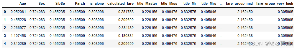
5.1LogisticRegression建模
##LogisticRegression建模

# import LogisticRegression model in python.
from sklearn.linear_model import LogisticRegression
from sklearn.metrics import mean_absolute_error, accuracy_score

## call on the model object
logreg = LogisticRegression(solver='liblinear',
                            penalty= 'l1',random_state = 42

                            )

## fit the model with "train_x" and "train_y"
logreg.fit(X_train,y_train)

y_pred = logreg.predict(X_test)

from sklearn.metrics import classification_report, confusion_matrix
# printing confision matrix
pd.DataFrame(confusion_matrix(y_test,y_pred),\
            columns=["Predicted Not-Survived", "Predicted Survived"],\
            index=["Not-Survived","Survived"] )

'''结果:
 	Predicted Not-Survived 	Predicted Survived
Not-Survived 	156 	           28
Survived 	     26 	           85
'''
from sklearn.metrics import classification_report, balanced_accuracy_score
print(classification_report(y_test, y_pred))
'''结果:
precision recall f1-score support
0 0.86 0.85 0.85 184
1 0.75 0.77 0.76 111
accuracy 0.82 295
macro avg 0.80 0.81 0.81 295
weighted avg 0.82 0.82 0.82 295
'''
from sklearn.metrics import accuracy_score
accuracy_score(y_test, y_pred)
#结果:0.81694915254237295.2Decision Tree建模
##Decision Tree建模
from sklearn.model_selection import RandomizedSearchCV
from sklearn.model_selection import GridSearchCV, StratifiedKFold, StratifiedShuffleSplit
from sklearn.model_selection import GridSearchCV
from sklearn.tree import DecisionTreeClassifier
max_depth = range(1,30)
max_feature = [21,22,23,24,25,26,28,29,30,'auto']
criterion=["entropy", "gini"]

param = {'max_depth':max_depth,
         'max_features':max_feature,
         'criterion': criterion}
grid = GridSearchCV(DecisionTreeClassifier(),
                                param_grid = param,
                                 verbose=False,
                                 cv=StratifiedShuffleSplit(n_splits=20, random_state=15),
                                n_jobs = -1)
grid.fit(X, y)


print( grid.best_params_)
print (grid.best_score_)
print (grid.best_estimator_)
'''结果:
{'criterion': 'entropy', 'max_depth': 5, 'max_features': 30}
0.828888888888889
DecisionTreeClassifier(criterion='entropy', max_depth=5, max_features=30)
'''

dectree_grid = grid.best_estimator_
## using the best found hyper paremeters to get the score. 最好的模型参数
dectree_grid.score(X,y)

#结果:0.8585858585858586
5.3randomforest建模
##randomforest建模
from sklearn.model_selection import GridSearchCV, StratifiedKFold, StratifiedShuffleSplit
from sklearn.ensemble import RandomForestClassifier
n_estimators = [140,145,150,155,160];
max_depth = range(1,10);
criterions = ['gini', 'entropy'];
cv = StratifiedShuffleSplit(n_splits=10, test_size=.30, random_state=15)


parameters = {'n_estimators':n_estimators,
              'max_depth':max_depth,
              'criterion': criterions

        }
grid = GridSearchCV(estimator=RandomForestClassifier(max_features='auto'),
                                 param_grid=parameters,
                                 cv=cv,
                                 n_jobs = -1)
grid.fit(X,y)

print (grid.best_score_)
print (grid.best_params_)
print (grid.best_estimator_)
'''结果:
0.8384328358208956
{'criterion': 'entropy', 'max_depth': 7, 'n_estimators': 160}
RandomForestClassifier(criterion='entropy', max_depth=7, max_features='auto',
                       n_estimators=160)
'''

rf_grid = grid.best_estimator_
rf_grid.score(X,y)
#结果:0.8742985409652076
5.4Adaboost建模
from sklearn.tree import DecisionTreeClassifier
from sklearn.ensemble import AdaBoostClassifier

# 创建一个决策树分类器作为基本估计器
base_estimator = DecisionTreeClassifier()

# 创建AdaBoost分类器并将决策树分类器作为基本估计器
ada_boost = AdaBoostClassifier(base_estimator=base_estimator)

# 使用AdaBoost分类器进行训练和预测
ada_boost.fit(X_train, y_train)

predictions = ada_boost.predict(X_test)

from sklearn.metrics import accuracy_score

accuracy_score(y_test, y_pred)
#结果:0.8169491525423729


from sklearn.model_selection import GridSearchCV
from sklearn.model_selection import StratifiedShuffleSplit

n_estimators = [80,100,140,145,150,160, 170,175,180,185];
cv = StratifiedShuffleSplit(n_splits=10, test_size=.30, random_state=15)
learning_r = [0.1,1,0.01,0.5]

parameters = {'n_estimators':n_estimators,
              'learning_rate':learning_r

        }

base_estimator = DecisionTreeClassifier()

grid = GridSearchCV(AdaBoostClassifier(base_estimator= base_estimator, ## If None, then the base estimator is a decision tree.
                                     ),
                                 param_grid=parameters,
                                 cv=cv,
                                 n_jobs = -1)
grid.fit(X,y)

ada_grid = grid.best_estimator_
ada_grid.score(X,y)
#结果:0.9887766554433222