一、模型微调
上篇文章我们通过搭建三层卷积模型,训练了花卉图像识别模型,最后经验证集验证后准确率大约为 75% ,本篇文章对该数据集进行优化,提高识别的准确度。本篇文章中对于数据集的读取强化不做过多的介绍了,大家可以参考上篇文章中的介绍,下面是上篇文章的地址:
https://blog.csdn.net/qq_43692950/article/details/128518757
深度学习模型应用于小型图像数据集场景下,一般由于数据量的局限性,导致模型提取特征有限,进而影响识别的准确度,一种常用且非常高效的优化方式便是使用预训练网络模型。将一个已在大型数据集(例如ImageNet)上训练好的模型作为基础模型。在此基础上对自己的数据集再进行训练,即使新的数据集和原始数据集完全不同的情况下也可以得到很好的特诊提取。
使用预训练网络有两种方法:特征提取(feature extraction)和微调模型(fine-tuning):
-
特征提取(feature extraction):使用预训练的优秀模型和权重来从新样本中提取特征,最后给到一个新的分类器,从头开始训练,之前的权重会随着反向传播进行修改。
-
微调模型(fine-tuning):使用预训练的优秀模型和权重来从新样本中提取特征,最后同样给到一个新的分类器,但不同的是预训练模型的全部或某些层的权重被冻结,不会随着反向传播进行修改,只是略微调整了模型结构,这种方式不会破坏训练模型。
一般我们选取模型,都是基于ImageNet 上预训练过的用于图像分类的模型,在 keras 中可以在 keras.applications 下拿到各种网络模型结构,例如 VGG16、VGG19、Xception、ResNet、ResNetV2、 ResNeXt、InceptionV3、MobileNet、MobileNetV2、DenseNet 等。这些模型都是基于ImageNet 1000 分类的模型。
下面是 keras 中对各个模型的介绍:
https://keras.io/zh/applications/
其中各个模型在 ImageNet 上的Top1 和 Top5 的准确率如下
| 模型 | 大小 | Top-1 准确率 | Top-5 准确率 | 参数数量 | 深度 |
|---|---|---|---|---|---|
| Xception | 88 MB | 0.790 | 0.945 | 22,910,480 | 126 |
| VGG16 | 528 MB | 0.713 | 0.901 | 138,357,544 | 23 |
| VGG19 | 549 MB | 0.713 | 0.900 | 143,667,240 | 26 |
| ResNet50 | 98 MB | 0.749 | 0.921 | 25,636,712 | - |
| ResNet101 | 171 MB | 0.764 | 0.928 | 44,707,176 | - |
| ResNet152 | 232 MB | 0.766 | 0.931 | 60,419,944 | - |
| ResNet50V2 | 98 MB | 0.760 | 0.930 | 25,613,800 | - |
| ResNet101V2 | 171 MB | 0.772 | 0.938 | 44,675,560 | - |
| ResNet152V2 | 232 MB | 0.780 | 0.942 | 60,380,648 | - |
| ResNeXt50 | 96 MB | 0.777 | 0.938 | 25,097,128 | - |
| ResNeXt101 | 170 MB | 0.787 | 0.943 | 44,315,560 | - |
| InceptionV3 | 92 MB | 0.779 | 0.937 | 23,851,784 | 159 |
| InceptionResNetV2 | 215 MB | 0.803 | 0.953 | 55,873,736 | 572 |
| MobileNet | 16 MB | 0.704 | 0.895 | 4,253,864 | 88 |
| MobileNetV2 | 14 MB | 0.713 | 0.901 | 3,538,984 | 88 |
| DenseNet121 | 33 MB | 0.750 | 0.923 | 8,062,504 | 121 |
| DenseNet169 | 57 MB | 0.762 | 0.932 | 14,307,880 | 169 |
| DenseNet201 | 80 MB | 0.773 | 0.936 | 20,242,984 201 | |
| NASNetMobile | 23 MB | 0.744 | 0.919 | 5,326,716 | - |
| NASNetLarge | 343 MB | 0.825 | 0.960 | 88,949,818 | - |
例如:查看 VGG16 模型的结构,其中如果权重文件不存在则会自动下载:
from tensorflow import keras

model = keras.applications.VGG16(weights='imagenet', include_top=True)
model.summary()
打印出下面内容,可以看出输入是 (224, 224, 3) 大小的三维图片,输出是一个 1000 分类的模型:
Model: "vgg16"
_________________________________________________________________
Layer (type)                 Output Shape              Param #
=================================================================
input_1 (InputLayer)         [(None, 224, 224, 3)]     0
_________________________________________________________________
block1_conv1 (Conv2D)        (None, 224, 224, 64)      1792
_________________________________________________________________
block1_conv2 (Conv2D)        (None, 224, 224, 64)      36928
_________________________________________________________________
block1_pool (MaxPooling2D)   (None, 112, 112, 64)      0
_________________________________________________________________
block2_conv1 (Conv2D)        (None, 112, 112, 128)     73856
_________________________________________________________________
block2_conv2 (Conv2D)        (None, 112, 112, 128)     147584
_________________________________________________________________
block2_pool (MaxPooling2D)   (None, 56, 56, 128)       0
_________________________________________________________________
block3_conv1 (Conv2D)        (None, 56, 56, 256)       295168
_________________________________________________________________
block3_conv2 (Conv2D)        (None, 56, 56, 256)       590080
_________________________________________________________________
block3_conv3 (Conv2D)        (None, 56, 56, 256)       590080
_________________________________________________________________
block3_pool (MaxPooling2D)   (None, 28, 28, 256)       0
_________________________________________________________________
block4_conv1 (Conv2D)        (None, 28, 28, 512)       1180160
_________________________________________________________________
block4_conv2 (Conv2D)        (None, 28, 28, 512)       2359808
_________________________________________________________________
block4_conv3 (Conv2D)        (None, 28, 28, 512)       2359808
_________________________________________________________________
block4_pool (MaxPooling2D)   (None, 14, 14, 512)       0
_________________________________________________________________
block5_conv1 (Conv2D)        (None, 14, 14, 512)       2359808
_________________________________________________________________
block5_conv2 (Conv2D)        (None, 14, 14, 512)       2359808
_________________________________________________________________
block5_conv3 (Conv2D)        (None, 14, 14, 512)       2359808
_________________________________________________________________
block5_pool (MaxPooling2D)   (None, 7, 7, 512)         0
_________________________________________________________________
flatten (Flatten)            (None, 25088)             0
_________________________________________________________________
fc1 (Dense)                  (None, 4096)              102764544
_________________________________________________________________
fc2 (Dense)                  (None, 4096)              16781312
_________________________________________________________________
predictions (Dense)          (None, 1000)              4097000
使用 VGG16 预测图片分类,图片如下:

from tensorflow import keras
import tensorflow as tf
import matplotlib.pyplot as plt
from tensorflow.keras.preprocessing.image import img_to_array
from tensorflow.keras.preprocessing.image import load_img

plt.rcParams['font.sans-serif'] = ['SimHei']

model = keras.applications.VGG16(weights='imagenet', include_top=True)

img_path = './img/cat.jpg'
image = load_img(img_path, target_size=(224, 224))
image = img_to_array(image)
# 预测
y_predictions = model.predict(tf.expand_dims(image, 0))
# 解析标签
y_lable = keras.applications.vgg16.decode_predictions(y_predictions)

plt.imshow(image / 255.0)
plt.title('预测结果:' + y_lable[0][0][1] + ',概率:' + str("%.2f" % (y_lable[0][0][2] * 100)) + '%')
plt.show()
预测结果:

二、使用 MobileNetV2 微调模型优化训练花卉图像识别
关于图像的预处理可以参考上篇文章,这里基于 MobileNetV2 模型进行微调,MobileNetV2 模型是一个轻量级的分类模型,由google团队在2018年提出的,相比MobileNet V1网络,准确率更高,模型更小,可用于移动端设置计算。
这里对 MobileNetV2 模型去除最后的分类器层,其余权重均被冻结,并在最后,加上两层全连接层和一层分类层,其中在 keras 中冻结参数,也非常容易,只需 Model.trainable = False 即可,例如:
mobienet = keras.applications.MobileNetV2(weights='imagenet', include_top=False, input_shape=(180, 180, 3))
 # 冻结权重
mobienet.trainable = False
整体模型如下所示:

下面使用 keras 构建模型结构:
import tensorflow as tf
from tensorflow import keras

# 定义模型类
class Model():
    # 初始化结构
    def __init__(self, checkpoint_path, log_path, model_path, num_classes, img_width, img_height):
        # checkpoint 权重保存地址
        self.checkpoint_path = checkpoint_path
        # 训练日志保存地址
        self.log_path = log_path
        # 训练模型保存地址:
        self.model_path = model_path

        # 数据统一大小并归一处理
        resize_and_rescale = tf.keras.Sequential([
            keras.layers.Resizing(img_width, img_height),
            keras.layers.Rescaling(1. / 255)
        ])
        # 数据增强
        data_augmentation = tf.keras.Sequential([
            # 翻转
            keras.layers.RandomFlip("horizontal_and_vertical"),
            # 旋转
            keras.layers.RandomRotation(0.2),
            # 对比度
            keras.layers.RandomContrast(0.3),
            # 随机裁剪
            # tf.keras.layers.RandomCrop(IMG_SIZE, IMG_SIZE),
            # 随机缩放
            keras.layers.RandomZoom(height_factor=0.3, width_factor=0.3),
        ])
        # MobileNetV2 模型结构
        mobienet = keras.applications.MobileNetV2(weights='imagenet', include_top=False, input_shape=(180, 180, 3))
        # 冻结权重
        mobienet.trainable = False
        # 初始化模型结构
        self.model = keras.Sequential([
            resize_and_rescale,
            data_augmentation,
            mobienet,
            keras.layers.Flatten(),
            keras.layers.Dense(1024,
                               kernel_initializer=keras.initializers.truncated_normal(stddev=0.05),
                               kernel_regularizer=keras.regularizers.l2(0.001),
                               activation=tf.nn.relu),
            keras.layers.Dense(256,
                               kernel_initializer=keras.initializers.truncated_normal(stddev=0.05),
                               kernel_regularizer=keras.regularizers.l2(0.001),
                               activation=tf.nn.relu),
            keras.layers.Dense(num_classes, activation='softmax')
        ])

    # 编译模型
    def compile(self):
        # 输出模型摘要
        self.model.build(input_shape=(None, 180, 180, 3))
        self.model.summary()
        # 定义训练模式
        self.model.compile(optimizer='adam',
                           loss='sparse_categorical_crossentropy',
                           metrics=['accuracy'])

    # 训练模型
    def train(self, train_ds, val_ds):
        # tensorboard 训练日志收集
        tensorboard = keras.callbacks.TensorBoard(log_dir=self.log_path)

        # 训练过程保存 Checkpoint 权重,防止意外停止后可以继续训练
        model_checkpoint = keras.callbacks.ModelCheckpoint(self.checkpoint_path,  # 保存模型的路径
                                                           # monitor='val_loss',  # 被监测的数据。
                                                           verbose=0,  # 详细信息模式,0 或者 1
                                                           save_best_only=True,  # 如果 True, 被监测数据的最佳模型就不会被覆盖
                                                           save_weights_only=True,
                                                           # 如果 True,那么只有模型的权重会被保存 (model.save_weights(filepath)),否则的话,整个模型会被保存,(model.save(filepath))
                                                           mode='auto',
                                                           # {auto, min, max}的其中之一。 如果 save_best_only=True,那么是否覆盖保存文件的决定就取决于被监测数据的最大或者最小值。 对于 val_acc,模式就会是 max,而对于 val_loss,模式就需要是 min,等等。 在 auto模式中,方向会自动从被监测的数据的名字中判断出来。
                                                           period=3  # 每3个epoch保存一次权重
                                                           )
        # 填充数据,迭代训练
        self.model.fit(
            train_ds,  # 训练集
            validation_data=val_ds,  # 验证集
            epochs=30,  # 迭代周期
            verbose=2,  # 训练过程的日志信息显示,一个epoch输出一行记录
            callbacks=[tensorboard, model_checkpoint]
        )
        # 保存训练模型
        self.model.save(self.model_path)

    def evaluate(self, val_ds):
        # 评估模型
        test_loss, test_acc = self.model.evaluate(val_ds)
        return test_loss, test_acc
处理数据集,其中使用 80% 的图像进行训练,20% 的图像进行验证。:
import tensorflow as tf
import pathlib
from tensorflow import keras

def getData():
    # 加载数据集
    path = "F:/Tensorflow/datasets/flower/flower_photos"
    # 解析目录
    data_dir = pathlib.Path(path)

    # keras 加载数据集
    batch_size = 20
    img_height = 180
    img_width = 180

    # 使用 80% 的图像进行训练,20% 的图像进行验证。
    class_names = ['daisy', 'dandelion', 'roses', 'sunflowers', 'tulips']
    train_ds = keras.utils.image_dataset_from_directory(
        data_dir,
        validation_split=0.2,
        subset="training",
        image_size=(img_height, img_width),
        batch_size=batch_size,
        shuffle=True,
        seed=123,
        interpolation='bilinear',
        crop_to_aspect_ratio=True,
        labels='inferred',
        class_names=class_names,
        color_mode='rgb'
    )

    val_ds = keras.utils.image_dataset_from_directory(
        data_dir,
        validation_split=0.2,
        subset="validation",
        image_size=(img_height, img_width),
        batch_size=batch_size,
        shuffle=True,
        seed=123,
        interpolation='bilinear',
        crop_to_aspect_ratio=True,
        labels='inferred',
        class_names=class_names,
        color_mode='rgb'
    )

    AUTOTUNE = tf.data.AUTOTUNE
    train_ds = train_ds.cache().prefetch(buffer_size=AUTOTUNE)
    val_ds = val_ds.cache().prefetch(buffer_size=AUTOTUNE)
    return train_ds, val_ds, len(class_names), img_width, img_height
开始训练模型:
def main():
    # 加载数据集
    train_ds, val_ds, num_classes, img_width, img_height = getData()

    checkpoint_path = './checkout/'
    log_path = './log'
    model_path = './model/model.h5'

    # 构建模型
    model = Model(checkpoint_path, log_path, model_path, num_classes, img_width, img_height)
    # 编译模型
    model.compile()
    # 训练模型
    model.train(train_ds, val_ds)
    # 评估模型
    test_loss, test_acc = model.evaluate(val_ds)
    print(test_loss, test_acc)

if __name__ == '__main__':
    main()
运行后可以看到打印的网络结构:

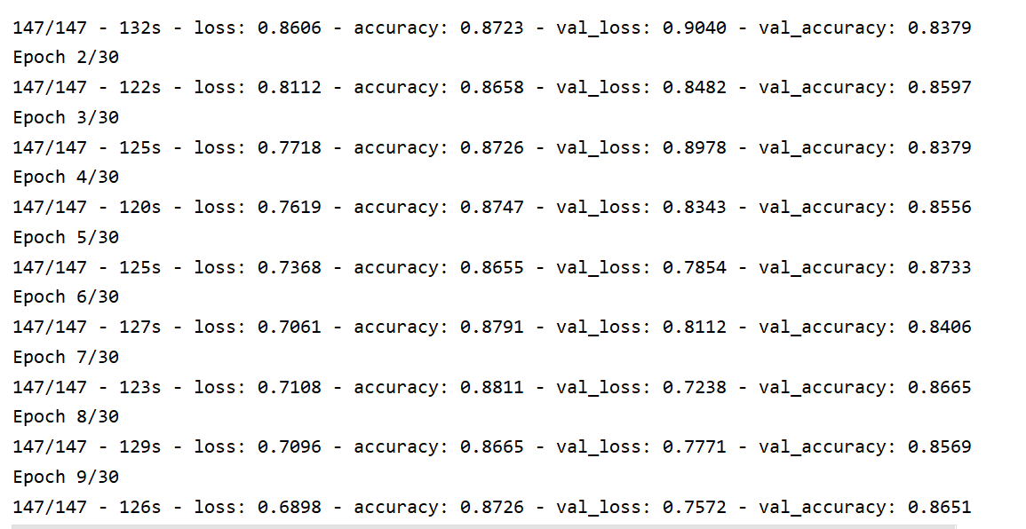
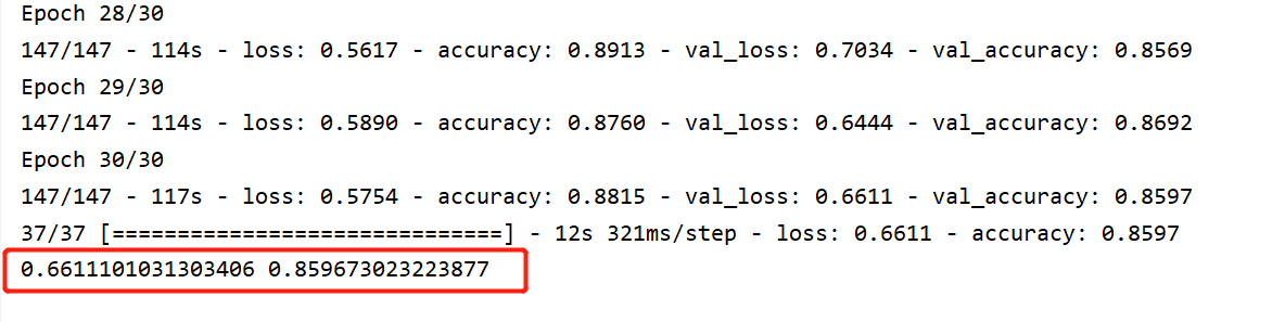
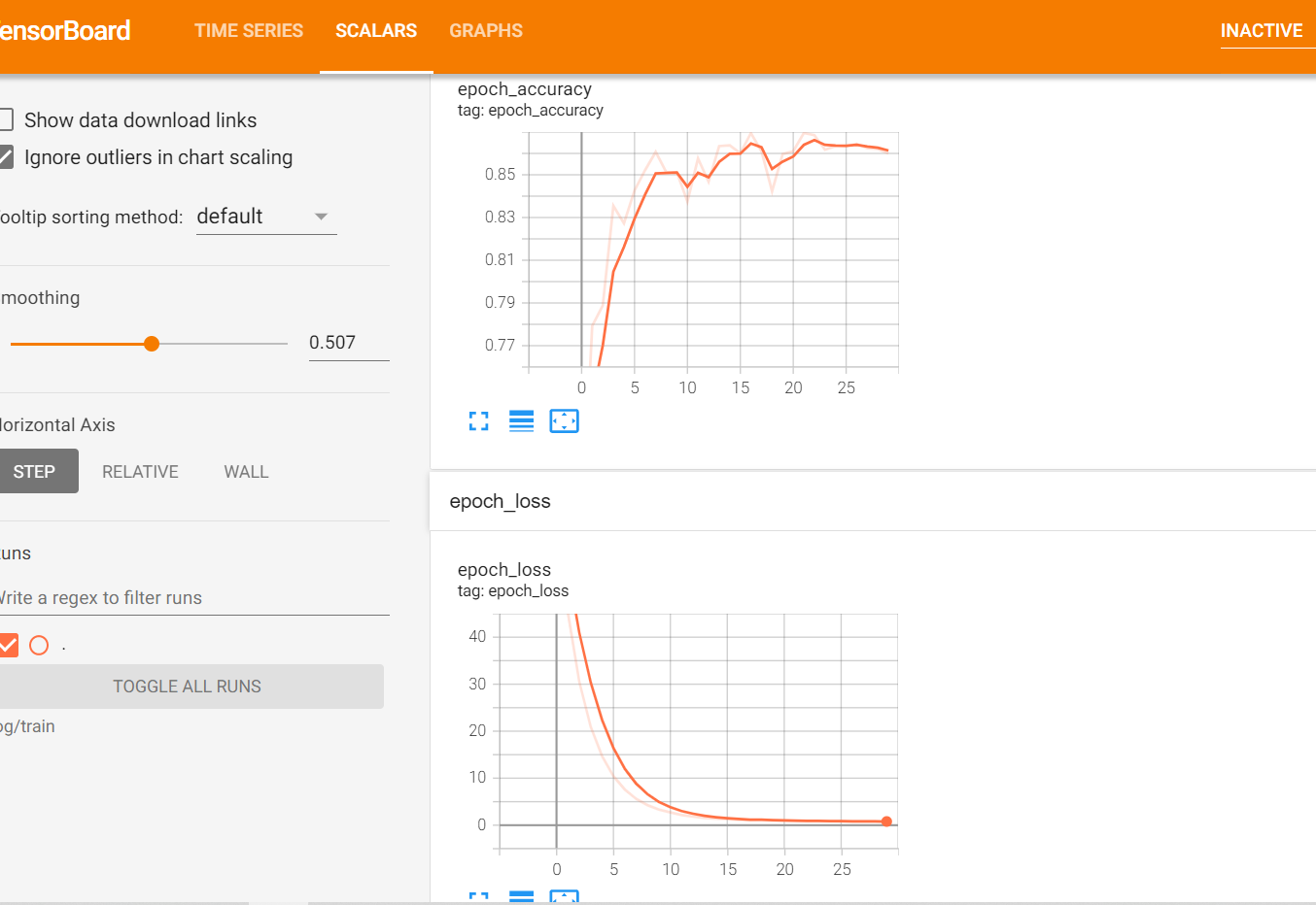
从训练日志中,可以看到 loss 一直在减小:
训练结束后评估模型的结果,最终在验证集上的准确率为: 85.96% ,比上篇文章整整高出了 10%
最后看下 tensorboard 中可视化的损失及准确率:
tensorboard --logdir=log/train
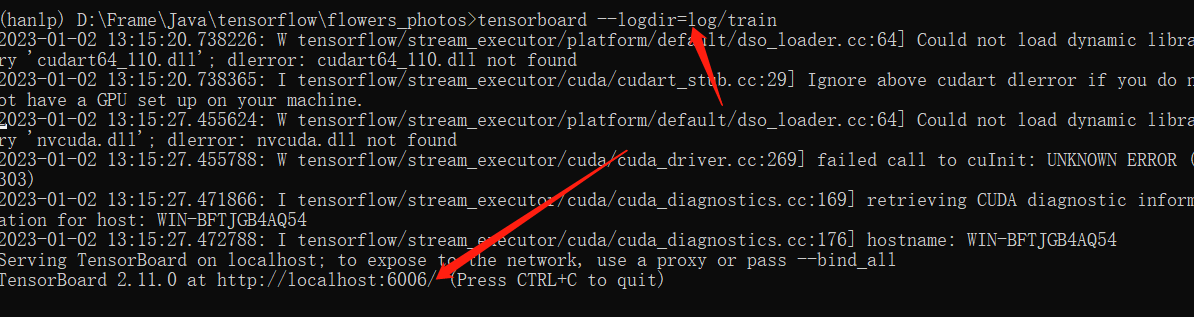
使用浏览器访问:http://localhost:6006/ 查看结果:
三、模型预测
训练后会在 model 下生成 model.h5 模型,下面直接加载该模型进行预测:
import tensorflow as tf
import pathlib
from tensorflow import keras
import matplotlib.pyplot as plt
plt.rcParams['font.sans-serif'] = ['SimHei']
def main():
# 加载数据集
path = "F:/Tensorflow/datasets/flower/flower_photos"
# 解析目录
data_dir = pathlib.Path(path)
# keras 加载数据集
batch_size = 32
img_height = 180
img_width = 180
class_names = ['daisy', 'dandelion', 'roses', 'sunflowers', 'tulips']
class_names_cn = ['雏菊', '蒲公英', '玫瑰', '向日葵', '郁金香']
val_ds = keras.utils.image_dataset_from_directory(
data_dir,
validation_split=0.2,
subset="validation",
image_size=(img_height, img_width),
batch_size=batch_size,
shuffle=True,
seed=123,
interpolation='bilinear',
crop_to_aspect_ratio=True,
labels='inferred',
class_names=class_names,
color_mode='rgb'
)
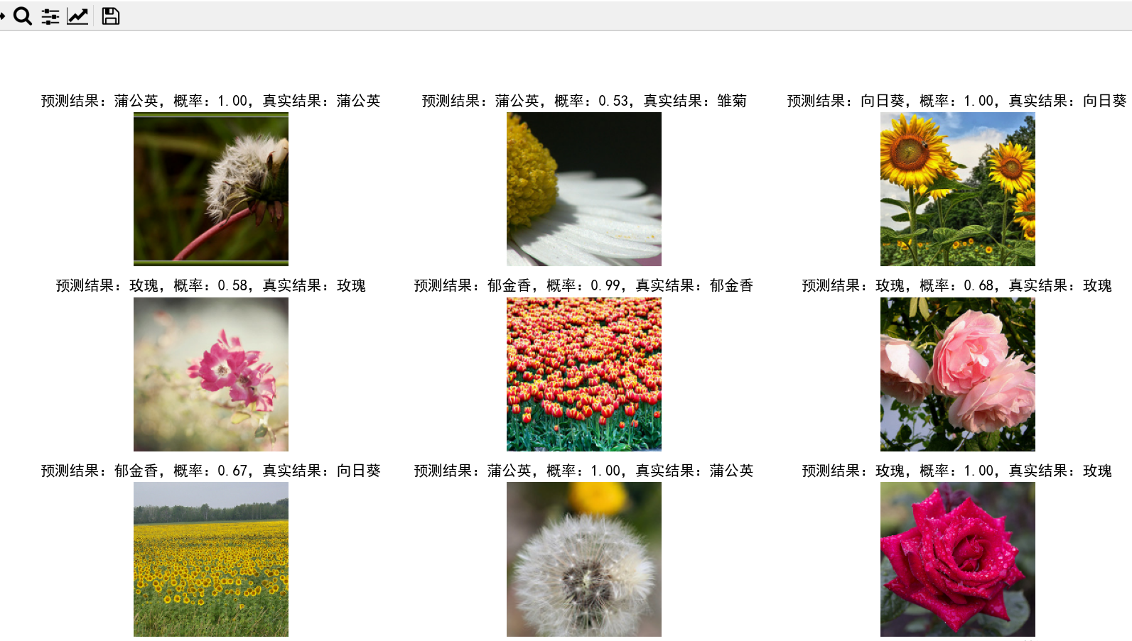
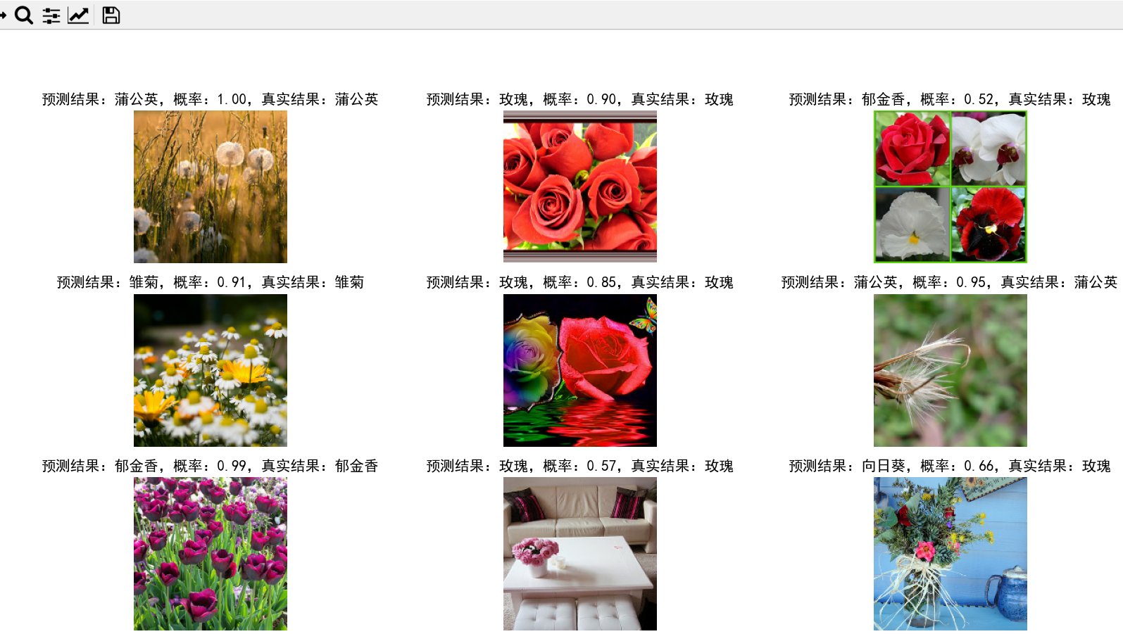
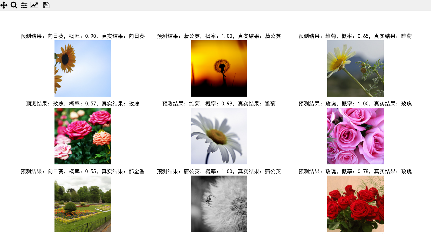
model = keras.models.load_model('./model/model.h5')
for image_batch, labels_batch in val_ds.take(3):
plt.figure(figsize=(10, 10))
for i in range(9):
plt.subplot(3, 3, i + 1)
softmax = model.predict(tf.expand_dims(image_batch[i], 0))
y_label = tf.argmax(softmax, axis=1).numpy()[0]
plt.imshow(image_batch[i].numpy().astype("uint8"))
plt.title('预测结果:' + class_names_cn[y_label] + ',概率:' + str("%.2f" % softmax[0][y_label]) + ',真实结果:' +
class_names_cn[labels_batch[i]])
plt.axis('off')
plt.show()
if __name__ == '__main__':
main()