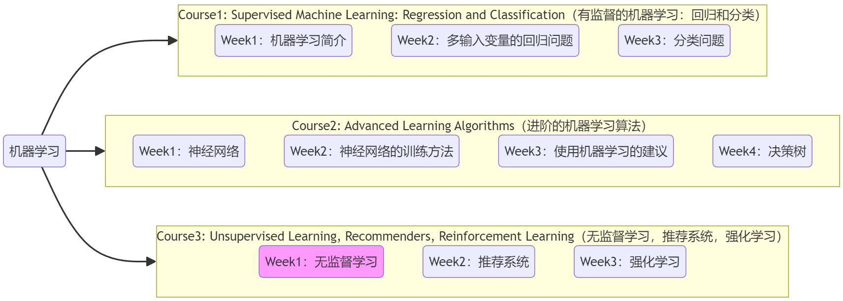
Course3-Week1-无监督学习

文章目录

Course3-Week1-无监督学习
- 1. 欢迎
- - 1.1 Course3简介
  - 1.2 数学符号约定
- 2. K-means算法
- 3. 异常检测
- - 3.1 异常检测的直观理解
  - 3.2 高斯分布
  - 3.3 异常检测算法
  - 3.4 选取判断阈值 $\varepsilon$
  - 3.5 选择恰当的特征
  - 3.6 异常检测与有监督学习对比
  - 3.7 代码实例-异常检测

笔记主要参考B站视频“(强推|双字)2022吴恩达机器学习Deeplearning.ai课程”。
该课程在Course上的页面：Machine Learning 专项课程
课程资料：“UP主提供资料(Github)”、或者“我的下载(百度网盘)”。
本篇笔记对应课程 Course3-Week1（下图中深紫色）。

1. 欢迎

1.1 Course3简介

前面的Course1、Course2一直在讨论“有监督的机器学习”，Course3就来介绍不一样的内容：

Week1-无监督机器学习(unsupervised learning)：主要学习“聚类(clustering)”及“异常检测(anomaly detection)”，这两种技术都广泛应用于商业软件中。
Week2-推荐机制(recommender systems)：“推荐系统”是机器学习最重要的商业应用之一，影响的产值达到数十亿美元，但在学术界却并没有取得相应的关注。常见于购物网站、流媒体视频等“为你推荐/猜你喜欢”的功能，学完后将理解广告的推荐策略。
Week3-强化学习(reinforcement learning)：“强化学习”是一项新的技术，和前面提到的技术相比，商业应用没有那么广泛。但这是一项令人兴奋的技术，它向人们展示了学习算法可以做的事情，比如打游戏、控制机器人等。课程最后将使用“强化学习”模拟一个月球着陆器。

1.2 数学符号约定

下面是本周会用到的数学符号，下面用到了再查就行。

数学符号约定：

样本数量为 $m$ 、特征的数量为 $n$ 、质心的数量为 $K$ 。
$\vec{x}^{(i)}$ ：是 $n$ 维向量，用于表示第 $i$ 个样本的位置。
$\vec{\mu}_k$ ：是 $n$ 维向量，用于表示第 $k$ 个质心的位置。
$c^{(i)}$ ：一个值，取值范围1~ $K$ ，表示第 $i$ 个样本 $\vec{x}^{(i)}$ 所对应的质心索引，该质心到 $\vec{x}^{(i)}$ 的欧式距离最短。
$\vec{\mu}_{c^{(i)}}$ ：表示第 $i$ 个样本 $\vec{x}^{(i)}$ 所对应的质心 $c^{(i)}$ 的位置。等价于 $\vec{\mu}_k$ ，只不过为了强调是 $\vec{x}^{(i)}$ 所对应的质心。
$\lVert x^{(i)}-\mu_k \rVert$ ：二阶范数，表示第 $i$ 个样本 $\vec{x}^{(i)}$ 和第 $k$ 个质心之间的欧式距离。但实际在代码中为减少计算量，通常使用该距离的平方，写成范数是为了数学形式的简便。
$\{ \vec{x}^{(1)};\vec{x}^{(2)};...;\vec{x}^{(n)} \}$ ：是 $m \times n$ 二维矩阵，每一行表示一个样本的位置。
$\Mu = \{ \vec{\mu}_1;\vec{\mu}_2;...;\vec{\mu}_K \}$ ：是 $K \times n$ 二维矩阵，每一行表示一个质心的位置。
$\vec{c} = \{ c^{(1)},c^{(2)},...,c^{(m)} \}$ ：是 $m$ 维向量，每个数都表示一个样本对应的质心索引。

注：上述中，“位置”向量中的每个参数都表示一个特征。
注：视频中老师没有标注向量符号，为了严谨且方便叙述，我标注上了。

2. K-means算法

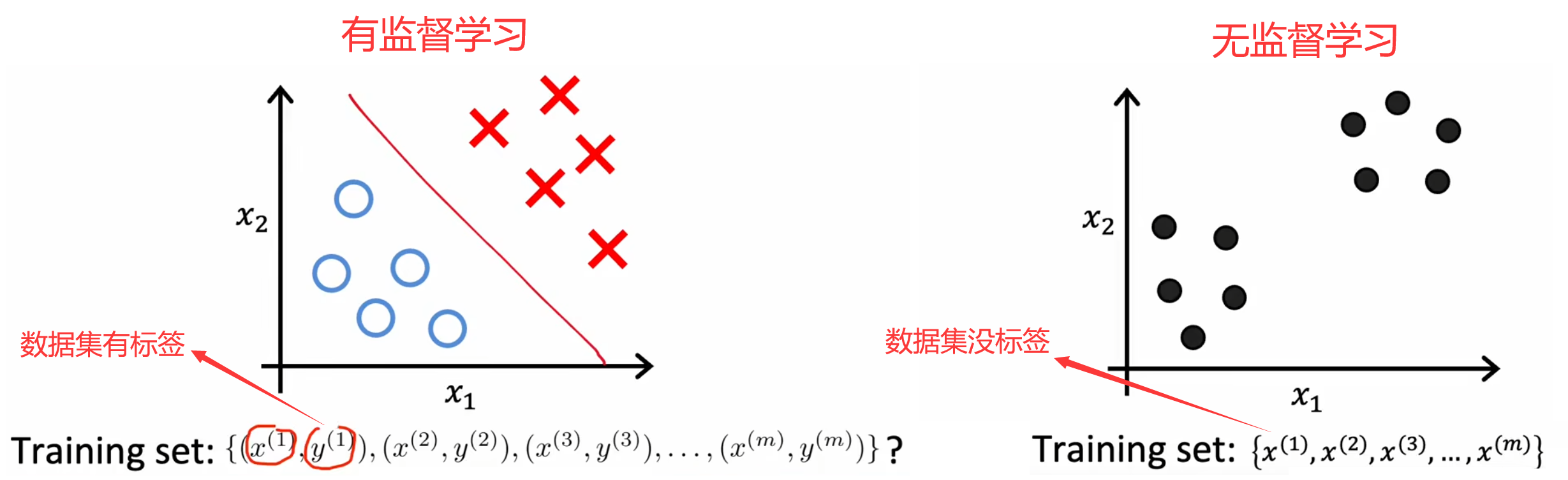
“聚类(clustering)”算法会自动将相似的数据点归为一类。和“有监督学习”不同，“聚类”这样的“无监督学习”算法的数据集没有标签。比如在Course1-Week1-2.2节中给出的一系列“无监督学习”示例：新闻分类、基因分类、客户分群、天文数据分析等。并且，“聚类”算法除了被用于有很明显分组的数据集，也可以对没有明显分组的数据集进行分类，比如设计T恤时的S、M、L尺码。

图3-1-1 有监督学习和无监督学习的数据集示意图

图3-1-2 没有明显分组的数据集

2.1 K-means算法的步骤

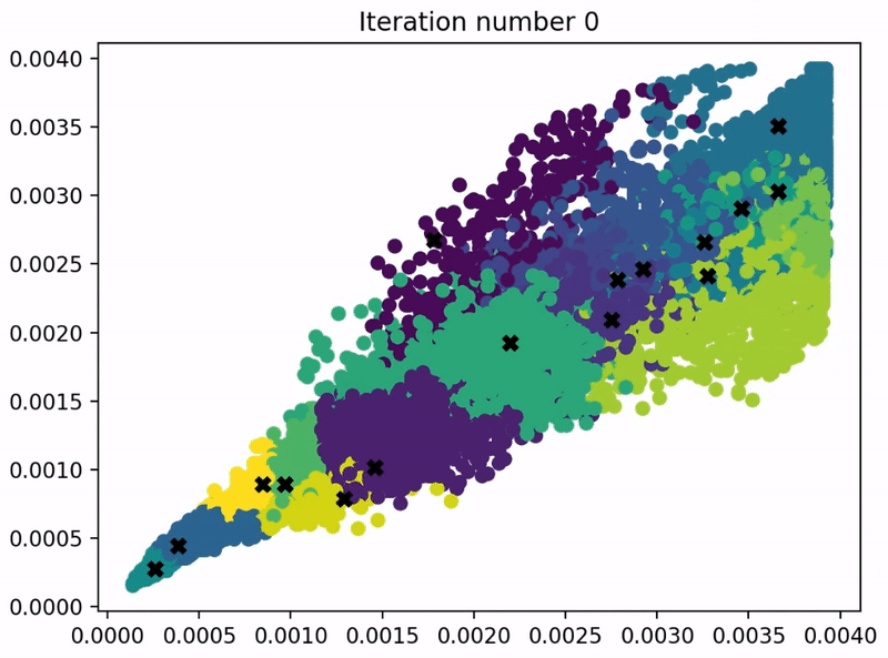
“K-means算法”是最常见的聚类算法，下面简单介绍一下“K-means算法”的原理。如下图所示，假设现在数据集中有30个未标记的训练样本，要求将数据分成两类。于是，我们可以先随机初始化两个“质心(centroid)”，然后不断的重复下面的步骤，直到质心的位置不再变化，也就是“收敛”：

为所有样本分配“质心”。也就是将当前样本，分配给距离最近的“质心”。
移动每一个“质心”。使用当前质心的所有样本计算出新的质心位置。

图3-1-3 K-means算法的直观理解

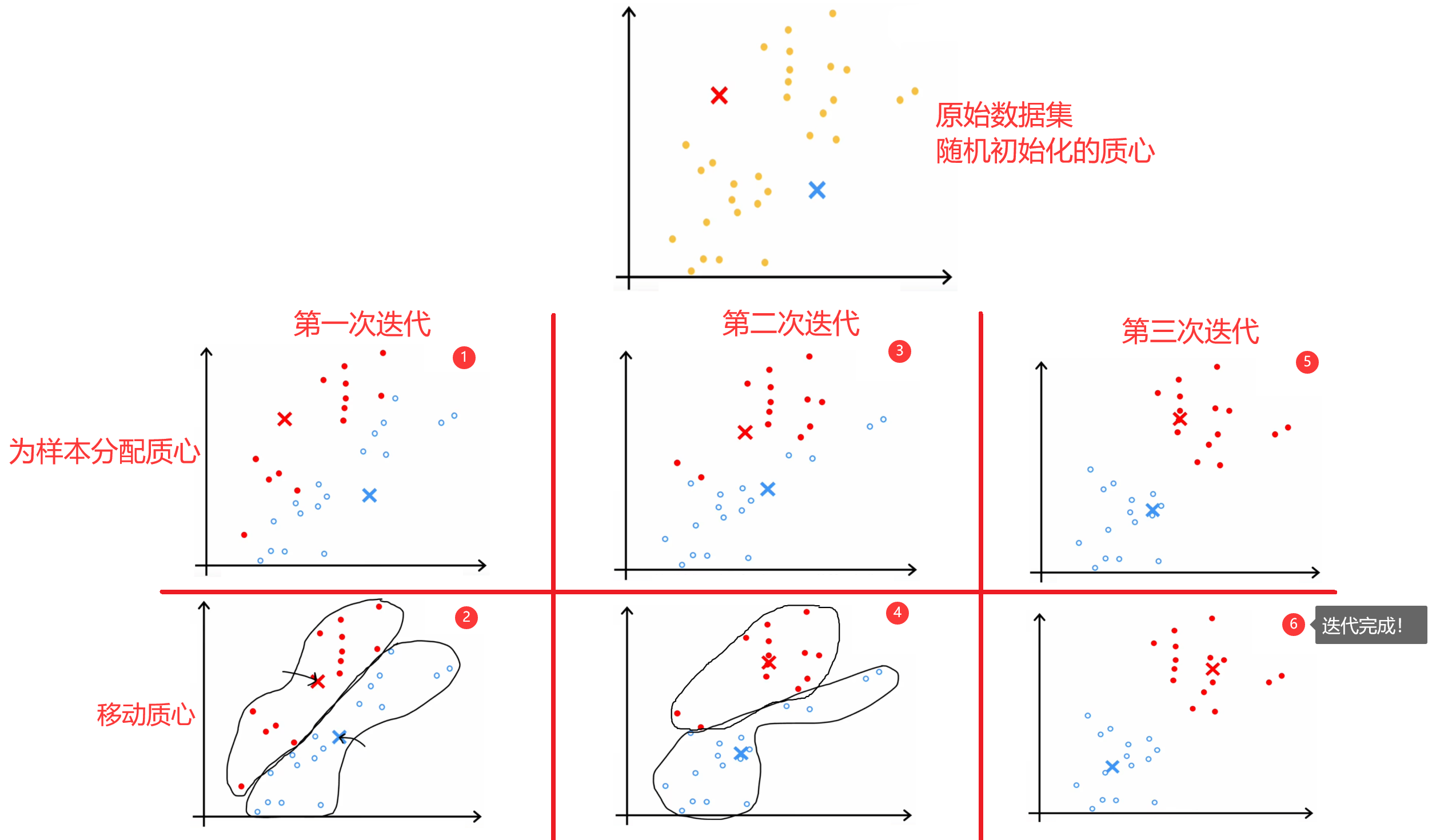
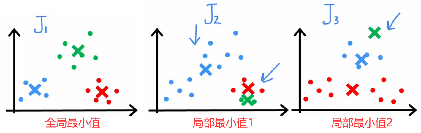
但“随机初始化”有一定的风险，因为不同的初始化会导致不同的聚类结果，所以很多迭代过程都会陷入到“局部最优解”中，如下图所示。所以解决方法就是将上述过程运行50~1000次，每次运行结束时都计算本次的代价函数，最终就可以找出代价最低的聚类结果。下面给出完整的“K-means算法”步骤：

图3-1-4 不同的初始化会导致不同的聚类结果

完整的K-means算法：

设定重复次数(如100次)：{
1. 随机选择 $K$ 个不同的样本作为 $K$ 个质心的初始位置： $\vec{\mu}_1,\vec{\mu}_2,...,\vec{\mu}_K$
2. 然后不断重复：{
1. 为样本分配质心。针对 $m$ 个样本，重复 $m$ 次，利用 $X$ 、 $\Mu$ 计算出距离当前样本最近的质心索引。最后得到 $\vec{c}$ 。
2. 移动质心。针对 $K$ 个质心，重复 $K$ 次，利用 $\vec{c}$ 计算出每个质心的新位置，并移动。质心的新位置等于该质心对应的所有样本位置的平均值。
}直到质心不再移动或移动步长很小(收敛)；
3. 计算并保存当前结果的代价。
}
找出代价最小的聚类结果。

注1：特征数量为 $n$ 、样本数量为 $m$ 、质心数量为 $K$ 。
注2：运行次数超过1000后，计算成本很高，但带来的收益很小，所以一般运行50~1000次即可。
注3：下一小节介绍“代价函数”的数学形式。

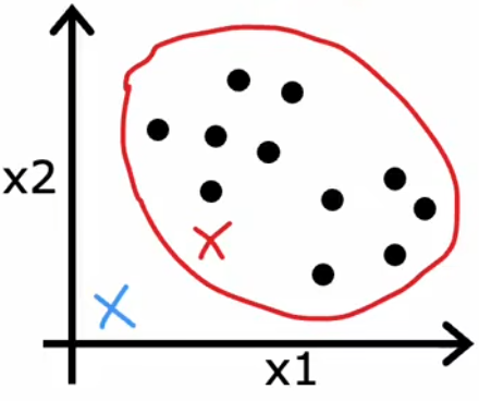
最后注意，若某次迭代结束后，某质心没有被分配到样本，如下图所示，那么：

去掉一个质心，也就是令 $K = K - 1$ 【常用】。
重新初始化质心位置，重新迭代。

图3-1-5 某质心没有被分配到样本

2.2 代价函数

上述介绍的整个“K-means算法”的过程，和“梯度下降法”相似，实质上也是在寻找特定代价函数的最小值。这个代价函数就是样本和其质点的距离的平方和的平均，在某些文献中也被称为“失真函数(distoration function)”：
$\begin{aligned} \text{Cost Function/} &\\ \text{Distoration Function}& \end{aligned}: J(\vec{c},\Mu) = \frac{1}{m}\sum_{i=1}^{m}\lVert x^{(i)}-\mu_{c^{(i)}} \rVert ^2$

所以，K-means算法实际上就是想让上述的距离的平均平方和最小。每次迭代中，代价函数都应该下降或不变，若代价不变或者下降的非常小则表明算法收敛，若代价上升则意味着代码有bug。

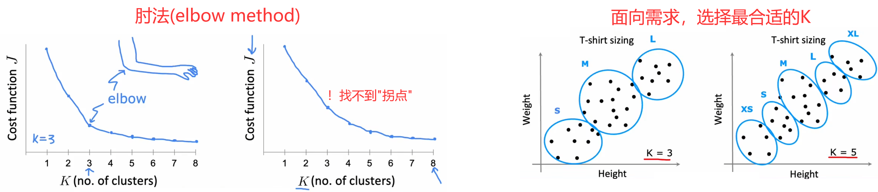
2.3 选择聚类数量

图3-1-6 聚类数量是一个主观的指标

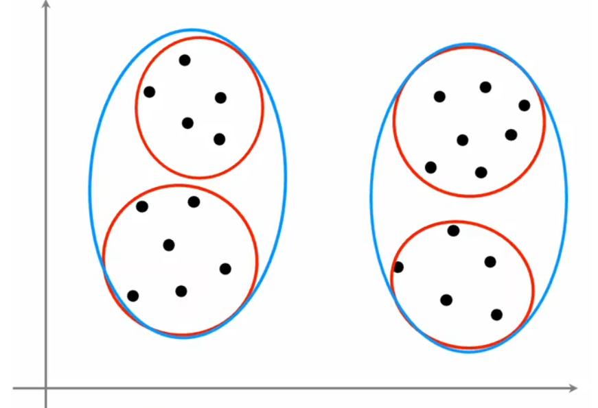
由于“K-means算法”属于“无监督学习”，所以聚类数量 $K$ 是很主观的指标，没有绝对正确的聚类数量。比如上图中，聚类数量是2、3、4，都非常合理。另外，聚类数量越多，代价函数的全局最小值越小，极端情况下令 $K = m$ ，此时每个样本都是一个类，显然代价为0最小。但通常来说，我们使用下面两种方法选择聚类数量 $K$ ：

“肘法(elbow method)”【不推荐】：画出代价函数的全局最小值 $J_{min}$ 随着 $K$ 变化的曲线，找出曲线“拐点(肘部)”所对应的 $K$ 作为最佳的聚类数量。但缺点是在大多数情况下，曲线都很平滑，找不到“拐点”。
面向需求【推荐】：通常当前的算法都会有后续的应用，所以可以根据应用需求选取相应的聚类数量。比如前面的“选择T恤尺码”问题，可以看设计需要选择3种尺码还是5种尺码，当然更多的尺码也意味着更多的成本，所以可以都运行一下，综合考虑最后结果再选择聚类数量。

图3-1-7 选择聚类数量的两种方法

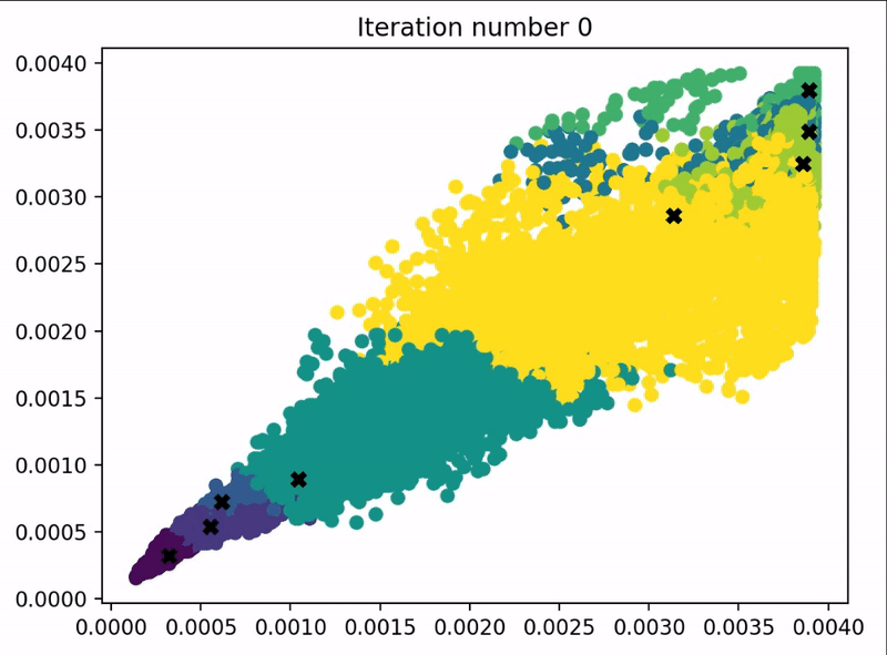
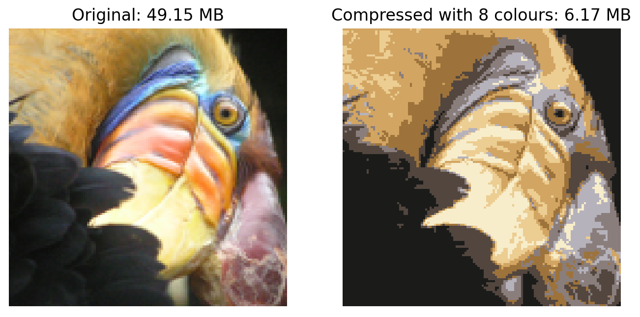
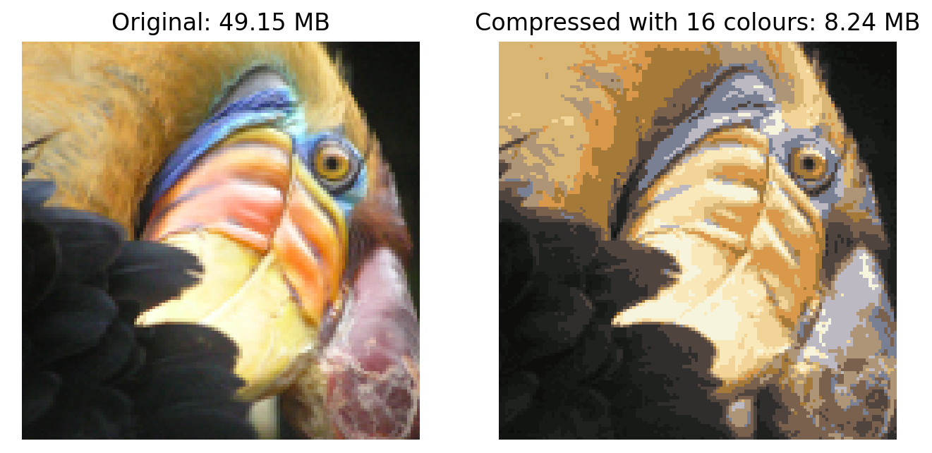
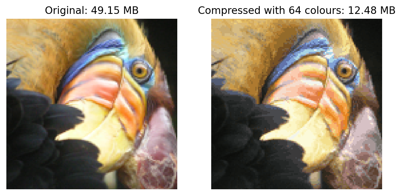
2.4 代码实例-图像压缩

本小节来使用K-means算法来实现图像压缩，问题要求和代码结构如下：

问题要求：使用K-means算法，找出下图最多的几种颜色，进行图像压缩。

代码结构：

函数：若干，后续再补充注释。
主函数：加载原始图像，运行K-means算法进行压缩，最后观察其和原图像的区别。

注：本实验来自本周的练习“C3_W1_KMeans_Assignment.ipynb”。

下面是代码和不同参数所对应的结果：

import numpy as np
import matplotlib.pyplot as plt
#################################################################
def plot_progress_kMeans(X, centroids, previous_centroids, idx, K, i):
    # 画出所有的样本点
    # plot_data_points(X, idx)
    plt.scatter(X[:, 0], X[:, 1], c=idx)
    # 画出当前的质心（黑色x）
    plt.scatter(centroids[:, 0], centroids[:, 1], marker='x', c='k', linewidths=3)
    # 将之前质心和当前质心连起来
    for j in range(centroids.shape[0]):
        plt.plot([centroids[j, :][0], previous_centroids[j, :][0]],
                 [centroids[j, :][1], previous_centroids[j, :][1]],
                 "-k", linewidth=1)
    plt.title("Iteration number %d" %i)
#################################################################
# 函数1：找到每个样本对应的最近的质心
def find_closest_centroids(X, centroids):
    """
    Computes the centroid memberships for every example    
    Args:
        X (ndarray): (m, n) Input values      
        centroids (ndarray): (k, n) values, k centroids
    Returns:
        idx (array_like): (m,) closest centroids
    """
    idx = np.zeros(X.shape[0], dtype=int)
    for i in range(X.shape[0]):
        idx[i] = (np.power(X[i]-centroids, 2)).sum(1).argmin()
    return idx
#################################################################
# 函数2：移动质心到新的位置
def compute_centroids(X, idx, K):
    """
    Returns the new centroids by computing the means of the 
    data points assigned to each centroid.
    Args:
        X (ndarray):   (m, n) Data points
        idx (ndarray): (m,) Array containing index of closest centroid for each 
                       example in X. Concretely, idx[i] contains the index of 
                       the centroid closest to example i
        K (int):       number of centroids
    Returns:
        centroids (ndarray): (K, n) New centroids computed
    """
    m, n = X.shape
    centroids = np.zeros((K, n))
    nums = np.zeros((K,1), dtype=int) # 每个质点所对应的样本数
    for i in range(m):
        centroids[idx[i]] += X[i]
        nums[idx[i]] += 1
    centroids = centroids/nums
    return centroids
#################################################################
# You do not need to implement anything for this part
def run_kMeans(X, initial_centroids, max_iters=10, plot_progress=False):
    """
    对数据集X运行k-Means算法，X的每一行是一个样本。
    """
    # 初始化参数
    m, n = X.shape
    K = initial_centroids.shape[0]
    centroids = initial_centroids
    previous_centroids = centroids    
    idx = np.zeros(m)
    # 运行K-Means
    for i in range(max_iters):
        # 输出当前迭代信息
        print("K-Means iteration %d/%d" % (i, max_iters-1))
        # 为每个样本分配最近的质心
        idx = find_closest_centroids(X, centroids)
        # Optionally plot progress
        if plot_progress:
            plot_progress_kMeans(X, centroids, previous_centroids, idx, K, i)
            plt.pause(1) # 防止更新太快，显示不出来
            previous_centroids = centroids
        # 移动质心位置
        centroids = compute_centroids(X, idx, K)
    # plt.show()
    return centroids, idx
#################################################################
# You do not need to modify this part
def kMeans_init_centroids(X, K):
    """
    在数据集X中，随机挑选K个样本作为初始的质心。    
    Args:
        X (ndarray): 数据集
        K (int):     质心的数量    
    Returns:
        centroids (ndarray): 初始化质心
    """
    randidx = np.random.permutation(X.shape[0])
    centroids = X[randidx[:K]]
    return centroids
#################################################################
# 加载原始图像
original_img = plt.imread('代码所在路径\\bird_small.png')
img_rows = original_img.shape[0]
img_cols = original_img.shape[1]
print("Shape of original_img is:", original_img.shape)

# Divide by 255 so that all values are in the range 0 - 1
original_img = original_img / 255

# Reshape the image into an m x 3 matrix where m = number of pixels
# (in this case m = 128 x 128 = 16384)
# Each row will contain the Red, Green and Blue pixel values
# This gives us our dataset matrix X_img that we will use K-Means on.
X_img = np.reshape(original_img, (original_img.shape[0] * original_img.shape[1], 3))

# Run your K-Means algorithm on this data
# You should try different values of K and max_iters here
K = 64
max_iters = 20

# Using the function you have implemented above. 
initial_centroids = kMeans_init_centroids(X_img, K) 

# Run K-Means - this takes a couple of minutes
# plt.figure()
# centroids, idx = run_kMeans(X_img, initial_centroids, max_iters, plot_progress=False) 
centroids, idx = run_kMeans(X_img, initial_centroids, max_iters, plot_progress=True) 

# 重新恢复出图片
X_recovered = centroids[idx, :] # 列向量
X_recovered = np.reshape(X_recovered, original_img.shape) # 图片向量
# 计算压缩前后的图片大小
original_byte = img_rows*img_cols*3
compress_byte = img_rows*img_cols*np.ceil(np.log2(K))/8 + K*3
# 显示原图
fig, ax = plt.subplots(1,2, figsize=(8,8))
plt.axis('off')
ax[0].imshow(original_img*255)
ax[0].set_title('Original: %.2f MB'%(original_byte/1000))
ax[0].set_axis_off()
# 显示压缩后的图片
ax[1].imshow(X_recovered*255)
ax[1].set_title('Compressed with %d colours: %.2f MB'%(K,compress_byte/1000))
ax[1].set_axis_off()
# 防止窗口自动关闭
plt.show(block=True)

图3-1-8 设置8个质心、迭代10次

图3-1-9 设置16个质心、迭代10次

图3-1-10 设置64个质心、迭代20次

本节 Quiz：

Which of these best describes unsupervised learning?
× A form of machine learning that finds patterns using labeled data (x,y).
× A form of machine learning that finds patterns in data using only labels (y) but without any inputs (x).
√ A form of machine learning that finds patterns using unlabeled data (x).
× A form of machine learning that finds patterns without using a cost function.

Which of these statements are true about K-means? Check all that apply.
√ If you are running K-means with $K = 3$ clusters, then each $c^{(i)}$ should be 1,2,or3.
√ If each example x is a vector of 5 numbers, then each cluster centroid $\mu_k$ is also going to be a vector of 5 numbers.
× The number of cluster centroids $\mu_k$ is equal to the number of examples.
√ The number of cluster assignment variables $c^{(i)}$ is equal to the number of training examples.

You run K-means 100 times with different initializations. How should you pick from the 100 resulting solutions?
× Pick the last one (i.e., the 100th random initialization) because K-means always improves over time.
× Average all 100 solutions together.
× Pick randomly - that was the point of random initialization.
√ Pick the one with the lowest cost $J$ .

You run K-means and compute the value of the cost function $J(c^{(1)},...,c^{(m)},\mu_1,...,\mu_k)$ after each iteration. Which of these statements should be true?
× Because K-means tries to maximize cost, the cost is always greater than or equal to the cost in the previous iteration.
× There is no cost function for the K-means algorithm.
× The cost can be greater or smaller than the cost in the previous iteration, but it decreases in the long run.
√ The cost will either decrease or stay the same after each iteration.

In K-means, the elbow method is a method to
× Choose the best number of samples in the dataset
× Choose the maximum number of examples for each cluster
× Choose the best random initialization
√ Choose the number of clusters K

3. 异常检测

下面来学习第二种商业应用广泛的“无监督学习”算法——“异常检测(anomaly detection)”。

3.1 异常检测的直观理解

【问题1】“飞机引擎检测”：根据输入特征，检测新制造的引擎是否有问题。

输入特征：“发动机温度”、“振动强度”。实际显然会有更多的特征，这里做出了简化。
输出：是否异常。
训练集： $m$ 个正常引擎的特征。

【问题2】“金融欺诈监测”：持续监测用户特征，判断是否有可能的欺诈行为。

输入特征：正常用户的登录频率、单次访问网页数量、单次交易数量、单次发帖数量、打字速度等。
输出：查看某个新用户是否具有欺诈行为。

【问题3】“服务器监测”：监测数据中心的服务器是否正常运行。

输入特征：内存使用量、磁盘读写次数、CPU负载、网络流量等。
输出：判断服务器是否出现异常行为，比如被黑客攻击等。

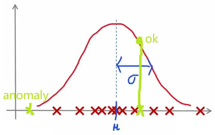
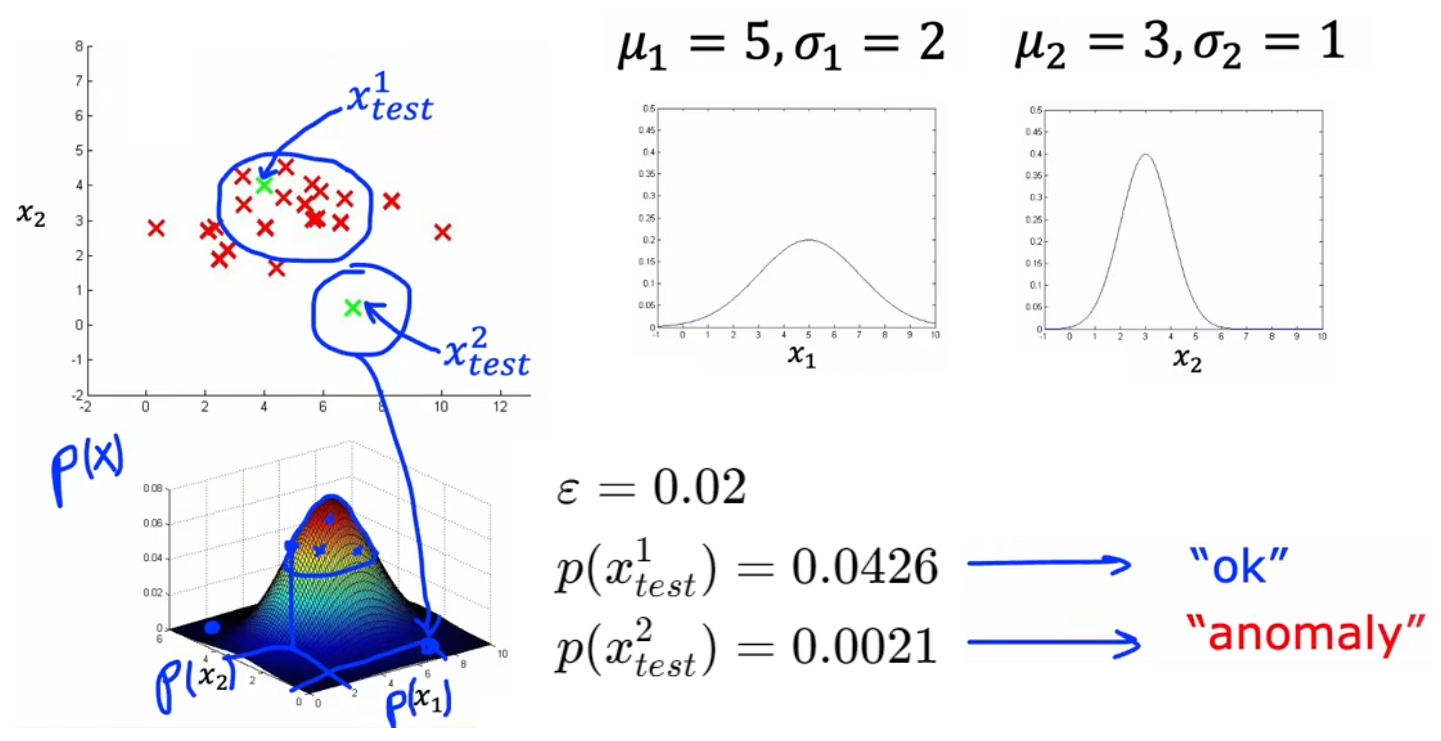
“异常检测”通常使用“(概率)密度估计(density estimation)”的方法。也就是，“异常检测”算法首先使用未标记的正常事件数据集进行训练(下图红叉)，学习正常样本的概率分布，然后计算新样本 $x_{test}$ 出现的概率，若其出现的概率小于设定好的阈值 $p(x_{test})<\varepsilon$ ，显然就可以认为这是一个异常事件：

图3-1-11 “异常检测”的直观理解

3.2 高斯分布

由于几乎所有从自然界采集的数据都服从高斯分布，所以我们使用高斯分布进行概率密度估计，本小节就来介绍“高斯分布(Gaussian distribution)”。下面是高斯分布的性质及表达式：

均值 $\mu$ 只是沿坐标轴平移曲线，不改变曲线形状。
方差 $\sigma^2$ 越大，曲线越扁平；方差 $\sigma^2$ 越小，曲线越集中。
概率和为1，所以 $\int_{-\infin}^{+\infin} p(x)dx=1$ 。
$3\sigma$ 原则： $x$ 出现在 $(\mu-3\sigma,\mu+3\sigma)$ 以外的概率小于 $0.3\%$ ，便认为是异常事件。根据精度要求，该标准可以在 $3\sigma\sim6\sigma$ 间浮动。

注：“高斯分布”别称“正态分布(Normal distribution)”、“钟形分布(Bell-shaped distribution)”，以下皆称“高斯分布”。

$\text{Gussion Distribution:}\quad p(x)=\frac{1}{\sqrt{2\pi}\sigma}e^{\frac{-(x-\mu)^2}{2\sigma^2}}$

图3-1-12 高斯分布

通过上述可以看到，高斯分布由均值 $\mu$ 和方差 $\sigma^2$ 完全确定。于是针对某单个特征，我们就可以计算其均值和方差，来对当前特征进行高斯估计(假设样本 $x^{(i)}$ 只有一个特征)：
$\mu = \frac{1}{m}\sum_{i=1}^m x^{(i)},\quad \sigma^2 = \frac{1}{m} \sum_{i=1}^m(x^{(i)}-\mu)^2.$

图3-1-13 使用高斯分布进行参数估计

3.3 异常检测算法

于是，根据上一节对单个特征进行高斯估计的公式，可以很容易的推广到具有多特征的样本，于是就可以写出下面“异常检测”算法的完整步骤。以3.1节的“飞机引擎检测”问题举例，首先使用正常样本分别对特征 $x_1$ 、 $x_2$ 进行概率统计，获得整体的概率统计后，就可以直接计算 $p(x_{test})$ 来判断其是否为异常事件：

“异常检测”算法的完整步骤：

定义训练集，注意全部为正常样本。假设样本总数为 $m$ 、特征总数为 $n$ 。
对每个特征分别进行统计分析，然后将其相乘得到某样本的综合概率分布。这里假设所有特征都服从高斯分布，并且相互独立。就算不独立，算法表现依旧良好：
$\mu_j = \frac{1}{m}\sum_{i=1}^m x^{(i)}_j,\quad \sigma^2_j = \frac{1}{m} \sum_{i=1}^m(x^{(i)}_j-\mu_j)^2, \quad j = 1,2,...,n.\\ p(\vec{x}) = p(x_1;\mu_1,\sigma^2_1)*p(x_2;\mu_2,\sigma^2_2)*...*p(x_n;\mu_n,\sigma^2_n) =\prod_{j=1}^n p(x_j;\mu_j,\sigma^2_j)$
对于新的输入 $\vec{x}_{new}$ ，代入 $p(\vec{x})$ 计算其概率。若 $p(\vec{x}_{new})<\varepsilon$ 则认为是异常事件。

图3-1-14 “异常检测”算法——飞机引擎检测

下一小节来介绍如何选取合适的判断阈值 $\varepsilon$ 。

3.4 选取判断阈值 $\varepsilon$

显然在开发系统时，如果有一个具体的评估系统性能的指标，就很容易帮助我们改进系统，这就是“实数评估(real-number evaluation)”。由于 $\varepsilon$ 也是“异常检测”的模型参数，于是这启示我们借鉴“有监督学习”中的“验证集”这一概念，来选择最合适的模型参数 $\varepsilon$ 。我们可以将“是否异常”看成是一种标签，来进行如下拆分，注意“训练集”是全部都为正常样本的无标签数据：

【异常样本足够】三拆分：训练集、验证集、测试集。

原始训练集：10000正常样本 + 20异常样本。
训练集：6000正常样本。用于拟合正常样本的概率分布。
验证集：2000正常样本+10异常样本。用于挑选最合适的 $\varepsilon$ 或者改进特征。
测试集：2000正常样本+10异常样本。用于最后评估系统性能。

【异常样本极少】二拆分：训练集、验证集。

原始训练集：10000正常样本 + 2异常样本。
训练集：6000正常样本。用于拟合正常样本的概率分布。
验证集：4000正常样本+2异常样本。用于挑选最合适的 $\varepsilon$ 或者改进特征。

注1：上述“二拆分”没有“测试集”评估系统性能，可能会有“过拟合”的风险。
注2：由于训练集没有标签，所以上述依旧是“无监督学习”。

进行上述拆分后，注意到上述“验证集”、“训练集”都属于Course2-Week3-第4节提到的“倾斜数据集”，于是就可以使用“准确率/召回率”、“F1 score”来评判系统在“验证集”、“测试集”上的性能。一个可行的代码思路是：

# 1. 训练结束后，计算验证集中所有样本对应的概率p_cv(0~1)。
# 2. 计算每个步长所对应的“F1 score”：
step = (max(p_cv) - min(p_cv)) / 1000
for epsilon in numpy.arange(min(p_cv), max(p_cv), step):
    # 计算当前 epsilon 下的“F1 score”
# 3. 找出最大的“F1 score”所对应的epsilon即可。

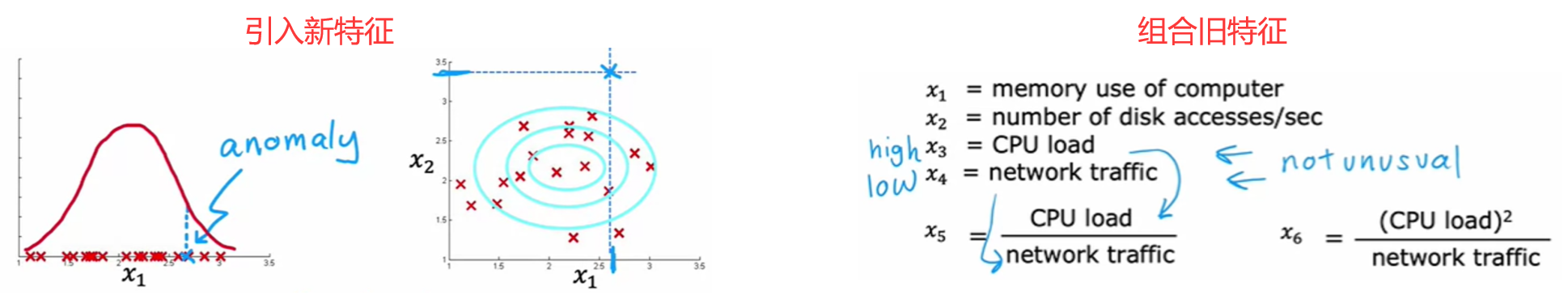
3.5 选择恰当的特征

在“有监督学习”中，即使选取的特征没那么恰当也没关系，因为算法可以从数据集的标签中学到如何重新缩放特征。但“无监督学习”的训练集没有标签，这就意味着 相比于“有监督学习”，选择恰当的特征对于“无监督学习”来说更重要。和前面类似，改进特征的方法主要有“特征变换”、“误差分析”：

特征变换：寻找更合适的概率分布

若原始特征不是高斯分布，那显然会引入很大的误差，于是：

进行特征变换(如下图)：通过数学变换将其变换成高斯分布。常见的改进方法有取对数 $\log(x+c)$ ， $c$ 为常数；幂次 $x^{n}$ ， $n$ 为任意实数。
使用其他分布进行拟合。如下图左侧就是“对数正态分布”，其他的还有“瑞利分布”、“指数分布”等。

注：上述两种方法原理相通，只不过方法二需要了解常见的统计分布。

图3-1-15 特征变换，使其为高斯分布

误差分析

如果在“验证集”上表现不佳，那么也可以进行“误差分析”，分析出现错误的原因，对症下药进行改进：

引入新特征：比如在“金融欺诈监测”中，检查某个被遗漏的异常样本，发现指标“交易次数 $x_1$ ”略高但在正常范围内，但是打字速度非常快，那么就可以添加新的特征“打字速度 $x_2$ ”。
组合旧特征：比如在“服务器监测”中，检查某个被遗漏的异常样本，所有指标都在合理范围内，只是“CPU负载 $x_3$ ”略高且“网络流量 $x_4$ ”略低，那么就可以组合这两个特征“CPU负载/网络流量 $x_5$ ”。

图3-1-16 改进特征的两种方法

3.6 异常检测与有监督学习对比

既然3.4节引入了“验证集”，将异常样本标记为1、正常样本标记为0，那为什么不使用前面的“有监督学习”完成检测异常样本的任务呢？这是因为两者的问题重心不同。总结一句话，“异常检测”尝试检测出“新异常”；“有监督学习”只检测“旧异常”。下面给出两者的对比：

异常检测-无监督学习：

异常样本极少。
异常的种类很多，异常样本无法覆盖到所有的异常；并且时常出现“新异常”。

如“金融欺诈监测”，每隔几个月都会出现全新的欺诈策略。
如“飞机引擎检测”，希望能检测到全新的缺陷。
如“服务器监测”，因为有人维护，所以黑客每次的入侵方式都不一样。许多系统安全相关的软件都使用“异常检测”。

有监督学习：

异常样本很多，甚至和正常样本一样多。
异常样本覆盖全面，以后出现的异常几乎都是之前出现过的。

如“垃圾邮件分类器”，内容无外乎保险、毒品、商品推销等。
如“产品缺陷检测”，流水线产品的缺陷几乎已经都是固定种类的，比如擦痕检测。
如“天气预报”，因为天气的种类是固定的：晴天、雨天等。
如“疾病检测”，看看病人是否有特定类型的疾病。

3.7 代码实例-异常检测

本小节完成对数据集的异常检测，问题要求和代码结构如下：

问题要求：完成对数据集的异常检测。
代码结构：

函数：若干，后续再补充注释。
主函数：加载原始数据集，运行检测算法，得到其最优的 $\varepsilon$ 。

注：本实验来自本周的练习“C3_W1_Anomaly_Detection.ipynb”。

下面是代码和输出结果：

import numpy as np
import matplotlib.pyplot as plt

#####################################################################
import numpy as np
import matplotlib.pyplot as plt

def load_data():
    X = np.load("C:/Users/14751/Desktop/机器学习-吴恩达/学习笔记/data/X_part1.npy")
    X_val = np.load("C:/Users/14751/Desktop/机器学习-吴恩达/学习笔记/data/X_val_part1.npy")
    y_val = np.load("C:/Users/14751/Desktop/机器学习-吴恩达/学习笔记/data/y_val_part1.npy")
    return X, X_val, y_val

def load_data_multi():
    X = np.load("C:/Users/14751/Desktop/机器学习-吴恩达/学习笔记/data/X_part2.npy")
    X_val = np.load("C:/Users/14751/Desktop/机器学习-吴恩达/学习笔记/data//X_val_part2.npy")
    y_val = np.load("C:/Users/14751/Desktop/机器学习-吴恩达/学习笔记/data//y_val_part2.npy")
    return X, X_val, y_val


def multivariate_gaussian(X, mu, var):
    """
    Computes the probability 
    density function of the examples X under the multivariate gaussian 
    distribution with parameters mu and var. If var is a matrix, it is
    treated as the covariance matrix. If var is a vector, it is treated
    as the var values of the variances in each dimension (a diagonal
    covariance matrix
    """
    
    k = len(mu)
    
    if var.ndim == 1:
        var = np.diag(var)
        
    X = X - mu
    p = (2* np.pi)**(-k/2) * np.linalg.det(var)**(-0.5) * \
        np.exp(-0.5 * np.sum(np.matmul(X, np.linalg.pinv(var)) * X, axis=1))
    
    return p
        
def visualize_fit(X, mu, var):
    """
    This visualization shows you the 
    probability density function of the Gaussian distribution. Each example
    has a location (x1, x2) that depends on its feature values.
    """
    
    X1, X2 = np.meshgrid(np.arange(0, 35.5, 0.5), np.arange(0, 35.5, 0.5))
    Z = multivariate_gaussian(np.stack([X1.ravel(), X2.ravel()], axis=1), mu, var)
    Z = Z.reshape(X1.shape)

    plt.plot(X[:, 0], X[:, 1], 'bx')

    if np.sum(np.isinf(Z)) == 0:
        plt.contour(X1, X2, Z, levels=10**(np.arange(-20., 1, 3)), linewidths=1)
        
    # Set the title
    plt.title("The Gaussian contours of the distribution fit to the dataset")
    # Set the y-axis label
    plt.ylabel('Throughput (mb/s)')
    # Set the x-axis label
    plt.xlabel('Latency (ms)')
#####################################################################
# UNQ_C1
# GRADED FUNCTION: estimate_gaussian

def estimate_gaussian(X): 
    """
    Calculates mean and variance of all features  in the dataset
    Args:
        X (ndarray): (m, n) Data matrix
    Returns:
        mu (ndarray): (n,) Mean of all features
        var (ndarray): (n,) Variance of all features
    """

    m, n = X.shape
    ### START CODE HERE ### 
    mu = X.mean(0)
    var = np.var(X,0)
    ### END CODE HERE ### 
        
    return mu, var

#####################################################################
# UNQ_C2
# GRADED FUNCTION: select_threshold

def select_threshold(y_val, p_val): 
    """
    Finds the best threshold to use for selecting outliers 
    based on the results from a validation set (p_val) 
    and the ground truth (y_val)
    
    Args:
        y_val (ndarray): Ground truth on validation set
        p_val (ndarray): Results on validation set
        
    Returns:
        epsilon (float): Threshold chosen 
        F1 (float):      F1 score by choosing epsilon as threshold
    """ 

    best_epsilon = 0
    best_F1 = 0
    F1 = 0
    
    step_size = (max(p_val) - min(p_val)) / 1000
    
    for epsilon in np.arange(min(p_val), max(p_val), step_size):
    
        ### START CODE HERE ### 
        y_bool = (y_val > 0.5)
        p_bool = (p_val < epsilon)
        tp = (p_bool & y_bool).sum()
        fp = (p_bool & (~y_bool)).sum()
        fn = ((~p_bool) & y_bool).sum()
        prec = 0 if (tp==0) else tp / (tp + fp)
        rec = 0 if (tp==0) else tp / (tp + fn)
        F1 = 0 if(prec==0 or rec==0) else 2*prec*rec/(prec+rec)
        ### END CODE HERE ### 
        
        if F1 > best_F1:
            best_F1 = F1
            best_epsilon = epsilon
        
    return best_epsilon, best_F1

#####################################################################
# Load the dataset
X_train, X_val, y_val = load_data()



# Create a scatter plot of the data. To change the markers to blue "x",
# we used the 'marker' and 'c' parameters
plt.scatter(X_train[:, 0], X_train[:, 1], marker='x', c='b') 

# Set the title
plt.title("The first dataset")
# Set the y-axis label
plt.ylabel('Throughput (mb/s)')
# Set the x-axis label
plt.xlabel('Latency (ms)')
# Set axis range
plt.axis([0, 30, 0, 30])
plt.show()

# Estimate mean and variance of each feature
mu, var = estimate_gaussian(X_train)   


# Returns the density of the multivariate normal
# at each data point (row) of X_train
p = multivariate_gaussian(X_train, mu, var)

#Plotting code 
visualize_fit(X_train, mu, var)


p_val = multivariate_gaussian(X_val, mu, var)
epsilon, F1 = select_threshold(y_val, p_val)

print('Best epsilon found using cross-validation: %e' % epsilon)
print('Best F1 on Cross Validation Set: %f' % F1)


# Find the outliers in the training set 
outliers = p < epsilon

# Visualize the fit
visualize_fit(X_train, mu, var)

# Draw a red circle around those outliers
plt.plot(X_train[outliers, 0], X_train[outliers, 1], 'ro',
         markersize= 10,markerfacecolor='none', markeredgewidth=2)



# 下面是高维数据
# load the dataset
X_train_high, X_val_high, y_val_high = load_data_multi()
print ('The shape of X_train_high is:', X_train_high.shape)
print ('The shape of X_val_high is:', X_val_high.shape)
print ('The shape of y_val_high is: ', y_val_high.shape)
# Apply the same steps to the larger dataset

# Estimate the Gaussian parameters
mu_high, var_high = estimate_gaussian(X_train_high)

# Evaluate the probabilites for the training set
p_high = multivariate_gaussian(X_train_high, mu_high, var_high)

# Evaluate the probabilites for the cross validation set
p_val_high = multivariate_gaussian(X_val_high, mu_high, var_high)

# Find the best threshold
epsilon_high, F1_high = select_threshold(y_val_high, p_val_high)

print('Best epsilon found using cross-validation: %e'% epsilon_high)
print('Best F1 on Cross Validation Set:  %f'% F1_high)
print('# Anomalies found: %d'% sum(p_high < epsilon_high))

Best epsilon found using cross-validation: 8.990853e-05
Best F1 on Cross Validation Set: 0.875000
The shape of X_train_high is: (1000, 11)
The shape of X_val_high is: (100, 11)
The shape of y_val_high is:  (100,)
Best epsilon found using cross-validation: 1.377229e-18
Best F1 on Cross Validation Set:  0.615385
# Anomalies found: 117

本节 Quiz：

You are building a system to detect if computers in a data center are malfunctioning. You have 10,000 data points of computers functioning well, and no data from computers malfunctioning. What type of algorithm should you use?
√ Anomaly detection
× Supervised learning

You are building a system to detect if computers in a data center are malfunctioning. You have 10,000 data points of computers functioning well, and 10,000 data points of computers malfunctioning. What type of algorithm should you use?
× Anomaly detection
√ Supervised learning

Say you have 5,000 examples of normal airplane engines, and 15 examples of anomalous engines. How would you use the 15 examples of anomalous engines to evaluate your anomaly detection algorithm?
× Because you have data of both normal and anomalous engines, don’t use anomaly detection. Use supervised learning instead.
× You cannot evaluate an anomaly detection algorithm because it is an unsupervised learning algorithm.
√ Put the data of anomalous engines (together with some normal engines) in the cross-validation and/or test sets to measure if the learned model can correctly detect anomalous engines.
× Use it during training by ftting one Gaussian model to the normal engines, and a different Gaussian model to the anomalous engines.

Anomaly detection flags a new input $x$ as an anomaly if $\varepsilon$ . If we reduce the value of $\varepsilon$ , what happens?
× The algorithm is more likely to classify new examples as an anomaly.
√ The algorithm is less likely to classify new examples as an anomaly.
× The algorithm is more likely to classify some examples as an anomaly, and less likely to classify some examples as an anomaly. It depends on the example $x$ .
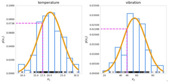
× The algorithm will automatically choose parameters $\mu$ and $\sigma$ to decrease $p (x)$ and compensate.

You are monitoring the temperature and vibration intensity on newly manufactured aircraft engines. You have measured 100 engines and fit the Gaussian model described in the video lectures to the data. The 100 examples and the resulting distributions are shown in the figure below.
The measurements on the latest engine you are testing have a temperature of 17.5 and a vibration intensity of 48. These are shown in magenta on the figure below. What is the probability of an engine having these two measurements?
Answer: 0.0738*0.02288 = 0.00169