本文仅供学习使用
本文参考:
B站:CLEAR_LAB
笔者带更新-运动学
课程主讲教师:
Prof. Wei Zhang
南科大高等机器人控制课 Ch02 Rigid Body Configuration and Velocity
- 1. Rigid Body Configuration
- 1.1 Special Orthogonal Group
- 1.2 Use of Rotation Matrix
- 1.3 Homogeneous Transformation Matrix
- 2. Rigid Body Velocity(Twist)
- 2.1 Rigid Body Velocity: Spatial Velocity (Twist)
- 2.2 Spatial Velocity Representation in a Reference Frame
- 2.3 Change Reference Frame for Twist
- 3. Geometric Aspect of Twist: Screw Motion
- 3.1 Screw Motion : Definition
- 3.2 From Screw Motion to Twist
- 3.3 From Twist to Screw Motion
- 3.4 Screw Reoersentation of a Twist
- 4. Extra Note : Tutorial on Twist/spatial Velocity and Screw Axis
- 4.1 What is Spatial Velocity and Twist
- 4.2 What is Screw Motion and Axis?
1. Rigid Body Configuration
- Free Vector
Free Vector: geometric quantity with length and direction
Given a reference frame, v ⃗ \vec{v} v can be move to a position such that the base of the arrow is at the origin without changing the orientation. Then the vector v ⃗ \vec{v} v can be represented by its coordinates v ⃗ \vec{v} v in the reference frame
v ⃗ \vec{v} v donated the physical quantity while v ⃗ A \vec{v}^A vA donate its coordinate wrt frame { A } \left\{ A \right\} {A}
Frame: coordinate system based on basis vectors—— { A : i ^ A , j ^ A , k ^ A } \left\{ A:\hat{i}^A,\hat{j}^A,\hat{k}^A \right\} {A:i^A,j^A,k^A}——3 coordinate vectors (unit length) i ^ A , j ^ A , k ^ A \hat{i}^A,\hat{j}^A,\hat{k}^A i^A,j^A,k^A and an origin
i
^
A
,
j
^
A
,
k
^
A
\hat{i}^A,\hat{j}^A,\hat{k}^A
i^A,j^A,k^A mutually orthogonal
i
^
A
×
j
^
A
=
k
^
A
\hat{i}^A\times \hat{j}^A=\hat{k}^A
i^A×j^A=k^A——right hand rule
- Point
Point : p p p denotes a point in the physical space
{
A
}
\left\{ A \right\}
{A} point
p
p
p can be represented by a vector from frame origin to
p
p
p
R
⃗
P
A
\vec{R}_{\mathrm{P}}^{A}
RPA denotes the coordinate of a point
p
p
p wrt frame
{
A
}
\left\{ A \right\}
{A}
此处使用了笔者习惯的表达方式,所以并不会出现不同坐标系下表达的向量不可相加的情况(本质并非坐标参数的相加),这种表达方式很多,本质都是为了简化直观向量表达的同时不产生歧义
- Cross Product
Cross Product or vector product of a ⃗ ∈ R 3 , b ⃗ ∈ R 3 \vec{a}\in \mathbb{R} ^3,\vec{b}\in \mathbb{R} ^3 a∈R3,b∈R3 is defined as
a ⃗ × b ⃗ = [ I ^ J ^ K ^ ] T [ a 2 b 3 − a 3 b 2 a 3 b 1 − a 1 b 3 a 1 b 2 − a 2 b 1 ] = [ I ^ J ^ K ^ ] T [ 0 − a 3 a 2 a 3 0 − a 1 − a 2 a 1 0 ] [ b 1 b 2 b 3 ] = [ I ^ J ^ K ^ ] T a ⃗ ~ [ b 1 b 2 b 3 ] \vec{a}\times \vec{b}=\left[ \begin{array}{c} \hat{I}\\ \hat{J}\\ \hat{K}\\ \end{array} \right] ^{\mathrm{T}}\left[ \begin{array}{c} a_2b_3-a_3b_2\\ a_3b_1-a_1b_3\\ a_1b_2-a_2b_1\\ \end{array} \right] =\left[ \begin{array}{c} \hat{I}\\ \hat{J}\\ \hat{K}\\ \end{array} \right] ^{\mathrm{T}}\left[ \begin{matrix} 0& -a_3& a_2\\ a_3& 0& -a_1\\ -a_2& a_1& 0\\ \end{matrix} \right] \left[ \begin{array}{c} b_1\\ b_2\\ b_3\\ \end{array} \right] =\left[ \begin{array}{c} \hat{I}\\ \hat{J}\\ \hat{K}\\ \end{array} \right] ^{\mathrm{T}}\tilde{\vec{a}}\left[ \begin{array}{c} b_1\\ b_2\\ b_3\\ \end{array} \right] a×b= I^J^K^ T a2b3−a3b2a3b1−a1b3a1b2−a2b1 = I^J^K^ T 0a3−a2−a30a1a2−a10 b1b2b3 = I^J^K^ Ta~ b1b2b3
a
⃗
~
=
−
a
⃗
~
T
\tilde{\vec{a}}=-\tilde{\vec{a}}^{\mathrm{T}}
a~=−a~T (called skew stmmetric)
a
⃗
~
b
⃗
~
−
b
⃗
~
a
⃗
~
=
a
⃗
×
b
⃗
~
\tilde{\vec{a}}\tilde{\vec{b}}-\tilde{\vec{b}}\tilde{\vec{a}}=\widetilde{\vec{a}\times \vec{b}}
a~b~−b~a~=a×b
Jocabi’s Idenetity
- Rotation Matrix
Rotation Matrix: specifies orientation of one frame relative to another
A valid rotation matrx [ Q B A ] \left[ Q_{\mathrm{B}}^{A} \right] [QBA] satisfies : [ Q B A ] [ Q B A ] T = E , det ( [ Q B A ] ) = 1 \left[ Q_{\mathrm{B}}^{A} \right] \left[ Q_{\mathrm{B}}^{A} \right] ^{\mathrm{T}}=E,\det \left( \left[ Q_{\mathrm{B}}^{A} \right] \right) =1 [QBA][QBA]T=E,det([QBA])=1
1.1 Special Orthogonal Group
Special Orthogonal Group : Space of Rotation Matrices in R n \mathbb{R} ^n Rn is defined as
S O ( n ) = { [ Q B A ] ∈ R n × n : [ Q B A ] [ Q B A ] T = E , det ( [ Q B A ] ) = 1 } SO\left( n \right) =\left\{ \left[ Q_{\mathrm{B}}^{A} \right] \in \mathbb{R} ^{n\times n}:\left[ Q_{\mathrm{B}}^{A} \right] \left[ Q_{\mathrm{B}}^{A} \right] ^{\mathrm{T}}=E,\det \left( \left[ Q_{\mathrm{B}}^{A} \right] \right) =1 \right\} SO(n)={[QBA]∈Rn×n:[QBA][QBA]T=E,det([QBA])=1}
S O ( n ) SO\left( n \right) SO(n) is a group. We are primarily interested in S O ( 3 ) SO\left( 3 \right) SO(3) and S O ( 2 ) SO\left( 2 \right) SO(2), rotation groups of R 3 \mathbb{R} ^3 R3 and R 2 \mathbb{R} ^2 R2 , respectively.
Group is a set G G G, together with an operation ∙ \bullet ∙, satisfying the following group
axioms/'æksɪəm/公理:
- Closure: a ∈ G , b ∈ G ⇒ a ∙ b ∈ G a\in G,b\in G\Rightarrow a\bullet b\in G a∈G,b∈G⇒a∙b∈G
- Assocaitivity: ( a ∙ b ) ∙ c = a ∙ ( b ∙ c ) , ∀ a , b , c ∈ G \left( a\bullet b \right) \bullet c=a\bullet \left( b\bullet c \right) ,\forall a,b,c\in G (a∙b)∙c=a∙(b∙c),∀a,b,c∈G
- Identity element: ∃ e ∈ G \exists e\in G ∃e∈G such that e ∙ a = a e\bullet a=a e∙a=a , for all a ∈ G a\in G a∈G
- Inverse element: For each a ∈ G a\in G a∈G, there is a b ∈ G b\in G b∈G such that a ∙ b = b ∙ a = e a\bullet b=b\bullet a=e a∙b=b∙a=e, where e e e is the identity element
1.2 Use of Rotation Matrix
- Representing an orientation —— from definition
将原矢量进行旋转变换,得到该坐标系下新矢量的坐标投影参数:
R ⃗ p ′ F = [ Q B A ] R ⃗ p F \vec{R}_{\mathrm{p}^{\prime}}^{F}=\left[ Q_{\mathrm{B}}^{A} \right] \vec{R}_{\mathrm{p}}^{F} Rp′F=[QBA]RpF - Changing the reference frame
对坐标系进行转换,基于坐标系 { B } \left\{ B \right\} {B}中的该矢量的坐标投影参数 R ⃗ p B \vec{R}_{\mathrm{p}}^{B} RpB,得到该矢量在坐标系 { A } \left\{ A \right\} {A}中的坐标投影参数 R ⃗ p A \vec{R}_{\mathrm{p}}^{A} RpA:
R ⃗ p A = [ Q B A ] R ⃗ p B \vec{R}_{\mathrm{p}}^{A}=\left[ Q_{\mathrm{B}}^{A} \right] \vec{R}_{\mathrm{p}}^{B} RpA=[QBA]RpB
[ i ⃗ B j ⃗ B k ⃗ B ] T [ P 1 B P 2 B P 3 B ] = [ i ⃗ A j ⃗ A k ⃗ A ] T [ P 1 A P 2 A P 3 A ] ⇒ ( [ Q B A ] T [ i ⃗ A j ⃗ A k ⃗ A ] ) T [ P 1 B P 2 B P 3 B ] = [ i ⃗ A j ⃗ A k ⃗ A ] T [ P 1 A P 2 A P 3 A ] ⇒ [ i ⃗ A j ⃗ A k ⃗ A ] T [ Q B A ] [ P 1 B P 2 B P 3 B ] = [ i ⃗ A j ⃗ A k ⃗ A ] T [ P 1 A P 2 A P 3 A ] ⇒ [ Q B A ] [ P 1 B P 2 B P 3 B ] = [ P 1 A P 2 A P 3 A ] = [ P ′ 1 B P ′ 2 B P ′ 3 B ] \left[ \begin{array}{c} \vec{i}^B\\ \vec{j}^B\\ \vec{k}^B\\ \end{array} \right] ^{\mathrm{T}}\left[ \begin{array}{c} P_{1}^{\mathrm{B}}\\ P_{2}^{\mathrm{B}}\\ P_{3}^{\mathrm{B}}\\ \end{array} \right] =\left[ \begin{array}{c} \vec{i}^A\\ \vec{j}^A\\ \vec{k}^A\\ \end{array} \right] ^{\mathrm{T}}\left[ \begin{array}{c} P_{1}^{A}\\ P_{2}^{A}\\ P_{3}^{A}\\ \end{array} \right] \\ \Rightarrow \left( \left[ Q_{\mathrm{B}}^{A} \right] ^{\mathrm{T}}\left[ \begin{array}{c} \vec{i}^A\\ \vec{j}^A\\ \vec{k}^A\\ \end{array} \right] \right) ^{\mathrm{T}}\left[ \begin{array}{c} P_{1}^{\mathrm{B}}\\ P_{2}^{\mathrm{B}}\\ P_{3}^{\mathrm{B}}\\ \end{array} \right] =\left[ \begin{array}{c} \vec{i}^A\\ \vec{j}^A\\ \vec{k}^A\\ \end{array} \right] ^{\mathrm{T}}\left[ \begin{array}{c} P_{1}^{A}\\ P_{2}^{A}\\ P_{3}^{A}\\ \end{array} \right] \\ \Rightarrow \left[ \begin{array}{c} \vec{i}^A\\ \vec{j}^A\\ \vec{k}^A\\ \end{array} \right] ^{\mathrm{T}}\left[ Q_{\mathrm{B}}^{A} \right] \left[ \begin{array}{c} P_{1}^{\mathrm{B}}\\ P_{2}^{\mathrm{B}}\\ P_{3}^{\mathrm{B}}\\ \end{array} \right] =\left[ \begin{array}{c} \vec{i}^A\\ \vec{j}^A\\ \vec{k}^A\\ \end{array} \right] ^{\mathrm{T}}\left[ \begin{array}{c} P_{1}^{A}\\ P_{2}^{A}\\ P_{3}^{A}\\ \end{array} \right] \\ \Rightarrow \left[ Q_{\mathrm{B}}^{A} \right] \left[ \begin{array}{c} P_{1}^{\mathrm{B}}\\ P_{2}^{\mathrm{B}}\\ P_{3}^{\mathrm{B}}\\ \end{array} \right] =\left[ \begin{array}{c} P_{1}^{A}\\ P_{2}^{A}\\ P_{3}^{A}\\ \end{array} \right] =\left[ \begin{array}{c} {P^{\prime}}_{1}^{\mathrm{B}}\\ {P^{\prime}}_{2}^{\mathrm{B}}\\ {P^{\prime}}_{3}^{\mathrm{B}}\\ \end{array} \right] iBjBkB T P1BP2BP3B = iAjAkA T P1AP2AP3A ⇒ [QBA]T iAjAkA T P1BP2BP3B = iAjAkA T P1AP2AP3A ⇒ iAjAkA T[QBA] P1BP2BP3B = iAjAkA T P1AP2AP3A ⇒[QBA] P1BP2BP3B = P1AP2AP3A = P′1BP′2BP′3B
- Rotating a vector or a frame (轴角变换)
Given two coordinate frames { A } \left\{ A \right\} {A} and { B } \left\{ B \right\} {B}, the configuration of B B B relative to A A A is determined by [ Q B A ] \left[ Q_{\mathrm{B}}^{A} \right] [QBA] and R ⃗ B A \vec{R}_{\mathrm{B}}^{A} RBA
For a (free) vector R ⃗ f r e e \vec{R}_{\mathrm{free}} Rfree, its coordinates R ⃗ f r e e A \vec{R}_{free}^{A} RfreeA and R ⃗ f r e e B \vec{R}_{free}^{B} RfreeB are related by : R ⃗ f r e e A = [ Q B A ] R ⃗ f r e e B \vec{R}_{free}^{A}=\left[ Q_{\mathrm{B}}^{A} \right] \vec{R}_{\mathrm{free}}^{B} RfreeA=[QBA]RfreeB
For a point P P P, its coordinates R ⃗ P A \vec{R}_{\mathrm{P}}^{A} RPA and R ⃗ P B \vec{R}_{\mathrm{P}}^{B} RPB are related by: R ⃗ P A = [ Q B A ] R ⃗ P B + R ⃗ B A \vec{R}_{\mathrm{P}}^{A}=\left[ Q_{\mathrm{B}}^{A} \right] \vec{R}_{\mathrm{P}}^{B}+\vec{R}_{\mathrm{B}}^{A} RPA=[QBA]RPB+RBA(一个无聊的小陷阱)
1.3 Homogeneous Transformation Matrix
Linear relation:
R
⃗
f
r
e
e
A
=
[
Q
B
A
]
R
⃗
f
r
e
e
B
\vec{R}_{\mathrm{free}}^{A}=\left[ Q_{\mathrm{B}}^{A} \right] \vec{R}_{\mathrm{free}}^{B}
RfreeA=[QBA]RfreeB——configuration of
{
B
}
\left\{ B \right\}
{B} relative to
{
A
}
\left\{ A \right\}
{A}
Affine relation:
R
⃗
P
A
=
[
Q
B
A
]
R
⃗
P
B
+
R
⃗
B
A
\vec{R}_{\mathrm{P}}^{A}=\left[ Q_{\mathrm{B}}^{A} \right] \vec{R}_{\mathrm{P}}^{B}+\vec{R}_{\mathrm{B}}^{A}
RPA=[QBA]RPB+RBA
Homogeneous Transformation Matrix: [ T B A ] \left[ T_{\mathrm{B}}^{A} \right] [TBA]
R ⃗ P A = [ Q B A ] R ⃗ P B + R ⃗ B A ⇒ [ R ⃗ P A 1 ] = [ [ Q B A ] R ⃗ B A 0 1 × 3 1 ] 4 × 4 [ R ⃗ P B 1 ] \vec{R}_{\mathrm{P}}^{A}=\left[ Q_{\mathrm{B}}^{A} \right] \vec{R}_{\mathrm{P}}^{B}+\vec{R}_{\mathrm{B}}^{A}\Rightarrow \left[ \begin{array}{c} \vec{R}_{\mathrm{P}}^{A}\\ 1\\ \end{array} \right] =\left[ \begin{matrix} \left[ Q_{\mathrm{B}}^{A} \right]& \vec{R}_{\mathrm{B}}^{A}\\ 0_{1\times 3}& 1\\ \end{matrix} \right] _{4\times 4}\left[ \begin{array}{c} \vec{R}_{\mathrm{P}}^{B}\\ 1\\ \end{array} \right] RPA=[QBA]RPB+RBA⇒[RPA1]=[[QBA]01×3RBA1]4×4[RPB1]
⇒ [ T B A ] = [ [ Q B A ] R ⃗ B A 0 1 ] \Rightarrow \left[ T_{\mathrm{B}}^{A} \right] =\left[ \begin{matrix} \left[ Q_{\mathrm{B}}^{A} \right]& \vec{R}_{\mathrm{B}}^{A}\\ 0& 1\\ \end{matrix} \right] ⇒[TBA]=[[QBA]0RBA1]
Homogeneous coordinates: Given a point P ∈ R 3 P\in \mathbb{R} ^3 P∈R3, its homogeneous coordinates is given by [ R ⃗ P A ] = [ R ⃗ P A 1 ] ∈ R 4 \left[ \vec{R}_{\mathrm{P}}^{A} \right] =\left[ \begin{array}{c} \vec{R}_{\mathrm{P}}^{A}\\ 1\\ \end{array} \right] \in \mathbb{R} ^4 [RPA]=[RPA1]∈R4
最终简化为:
[
R
⃗
P
A
]
=
[
T
B
A
]
[
R
⃗
P
B
]
\left[ \vec{R}_{\mathrm{P}}^{A} \right] =\left[ T_{\mathrm{B}}^{A} \right] \left[ \vec{R}_{\mathrm{P}}^{B} \right]
[RPA]=[TBA][RPB]
对于向量 R ⃗ P 1 P 2 A \vec{R}_{\mathrm{P}_1\mathrm{P}_2}^{A} RP1P2A 而言,则有:
[ R ⃗ P 1 P 2 A ] = [ R ⃗ P 2 A − R ⃗ P 1 A ] = [ R ⃗ P 2 A 1 ] − [ R ⃗ P 1 A 1 ] = [ R ⃗ P 2 A − R ⃗ P 1 A 0 ] = [ R ⃗ P 1 P 2 A 0 ] \left[ \vec{R}_{\mathrm{P}_1\mathrm{P}_2}^{A} \right] =\left[ \vec{R}_{\mathrm{P}_2}^{A}-\vec{R}_{\mathrm{P}_1}^{A} \right] =\left[ \begin{array}{c} \vec{R}_{\mathrm{P}_2}^{A}\\ 1\\ \end{array} \right] -\left[ \begin{array}{c} \vec{R}_{\mathrm{P}_1}^{A}\\ 1\\ \end{array} \right] =\left[ \begin{array}{c} \vec{R}_{\mathrm{P}_2}^{A}-\vec{R}_{\mathrm{P}_1}^{A}\\ 0\\ \end{array} \right] =\left[ \begin{array}{c} \vec{R}_{\mathrm{P}_1\mathrm{P}_2}^{A}\\ 0\\ \end{array} \right] [RP1P2A]=[RP2A−RP1A]=[RP2A1]−[RP1A1]=[RP2A−RP1A0]=[RP1P2A0]
- Example of Homogeneous Transformation Matrix

2. Rigid Body Velocity(Twist)
Consider a rigid body with angular velocity:
ω
⃗
\vec{\omega}
ω (this is a free vector)
Suppose the actual rotation axis passes through a point:
P
P
P ; Let
v
⃗
P
\vec{v}_{\mathrm{P}}
vP be the velocity of the point
P
P
P
- Question: A rigid body cibraubs infinitely many points with different velocities. How to
parameterize/pə'ræmɪtə,raɪz/参数化all of their velocities?
1.Consider an aritrary body-fixed point Q Q Q (means that the point is rigidly attached to the body, and moves with the body), we have: v ⃗ Q = v ⃗ P + ω ⃗ × R ⃗ P Q \vec{v}_{\mathrm{Q}}=\vec{v}_{\mathrm{P}}+\vec{\omega}\times \vec{R}_{\mathrm{PQ}} vQ=vP+ω×RPQ
2.The velocity of an arbitrary body-fixed point depends only on ( ω ⃗ , v ⃗ P , R ⃗ P \vec{\omega},\vec{v}_{\mathrm{P}},\vec{R}_{\mathrm{P}} ω,vP,RP) and the location of the point Q Q Q - Fact: The representation form is independent of the reference point P P P
- Consider an arbitrary point
S
S
S in space
1. S S S may not be on the rotation axis
2. S S S may be a stationary point in space(does not move)
3.Let v ⃗ S \vec{v}_{\mathrm{S}} vS be the velocity of the body-fixed point(rigidly attached to the body ) currently coincides with S S S(may not be body frame)
4.We still have: v ⃗ Q = v ⃗ P + ω ⃗ × R ⃗ P Q , v ⃗ S = v ⃗ P + ω ⃗ × R ⃗ P S ⇒ v ⃗ Q = v ⃗ S − ω ⃗ × R ⃗ P S + ω ⃗ × R ⃗ P Q = v ⃗ S + ω ⃗ × R ⃗ S Q \vec{v}_{\mathrm{Q}}=\vec{v}_{\mathrm{P}}+\vec{\omega}\times \vec{R}_{\mathrm{PQ}},\vec{v}_{\mathrm{S}}=\vec{v}_{\mathrm{P}}+\vec{\omega}\times \vec{R}_{\mathrm{PS}}\Rightarrow \vec{v}_{\mathrm{Q}}=\vec{v}_{\mathrm{S}}-\vec{\omega}\times \vec{R}_{\mathrm{PS}}+\vec{\omega}\times \vec{R}_{\mathrm{PQ}}=\vec{v}_{\mathrm{S}}+\vec{\omega}\times \vec{R}_{\mathrm{SQ}} vQ=vP+ω×RPQ,vS=vP+ω×RPS⇒vQ=vS−ω×RPS+ω×RPQ=vS+ω×RSQ
The body can be regarded as translating with a linear velocity v ⃗ S \vec{v}_{\mathrm{S}} vS , while rotating with angular velocity ω ⃗ \vec{\omega} ω about an axis passing through S S S
2.1 Rigid Body Velocity: Spatial Velocity (Twist)
-
Spatial Velocity(Twist) : V S = ( ω ⃗ , v ⃗ S ) \mathcal{V} _S=\left( \vec{\omega},\vec{v}_{\mathrm{S}} \right) VS=(ω,vS)
ω ⃗ \vec{\omega} ω - angular velocity; v ⃗ S \vec{v}_{\mathrm{S}} vS - velocity of the body-fixed point currently coincides with S S S
For any other body-fixed point Q Q Q, its velocity is v ⃗ Q = v ⃗ S + ω ⃗ × R ⃗ S Q \vec{v}_{\mathrm{Q}}=\vec{v}_{\mathrm{S}}+\vec{\omega}\times \vec{R}_{\mathrm{SQ}} vQ=vS+ω×RSQ -
Twist is a ‘physical’ quantity (just like linear or angular velocity): It can be represented in any chosen reference point S S S
-
A rigid body with V S = ( ω ⃗ , v ⃗ S ) \mathcal{V} _S=\left( \vec{\omega},\vec{v}_{\mathrm{S}} \right) VS=(ω,vS) can be ‘thought of’ as translating at v ⃗ S \vec{v}_{\mathrm{S}} vS while rotating with angular velocity ω ⃗ \vec{\omega} ω about an axis passing through S S S : This is just one way to interpret the motion.
2.2 Spatial Velocity Representation in a Reference Frame
Given frame { O } \left\{ O \right\} {O} and a spatial velocity V ∈ R 6 \mathcal{V} \in \mathbb{R} ^6 V∈R6
Choose o o o (the origin of { O } \left\{ O \right\} {O}) as the reference point to represent the rigid body velocity—— V O = ( ω ⃗ O , v ⃗ O ) \mathcal{V} ^O=\left( \vec{\omega}^O,\vec{v}^O \right) VO=(ωO,vO) : Coordinates for the V \mathcal{V} V in { O } \left\{ O \right\} {O} , by dafault, we assume the origin of the frame is used as the reference point: V O = V O O \mathcal{V} ^O=\mathcal{V} _{\mathrm{O}}^{O} VO=VOO
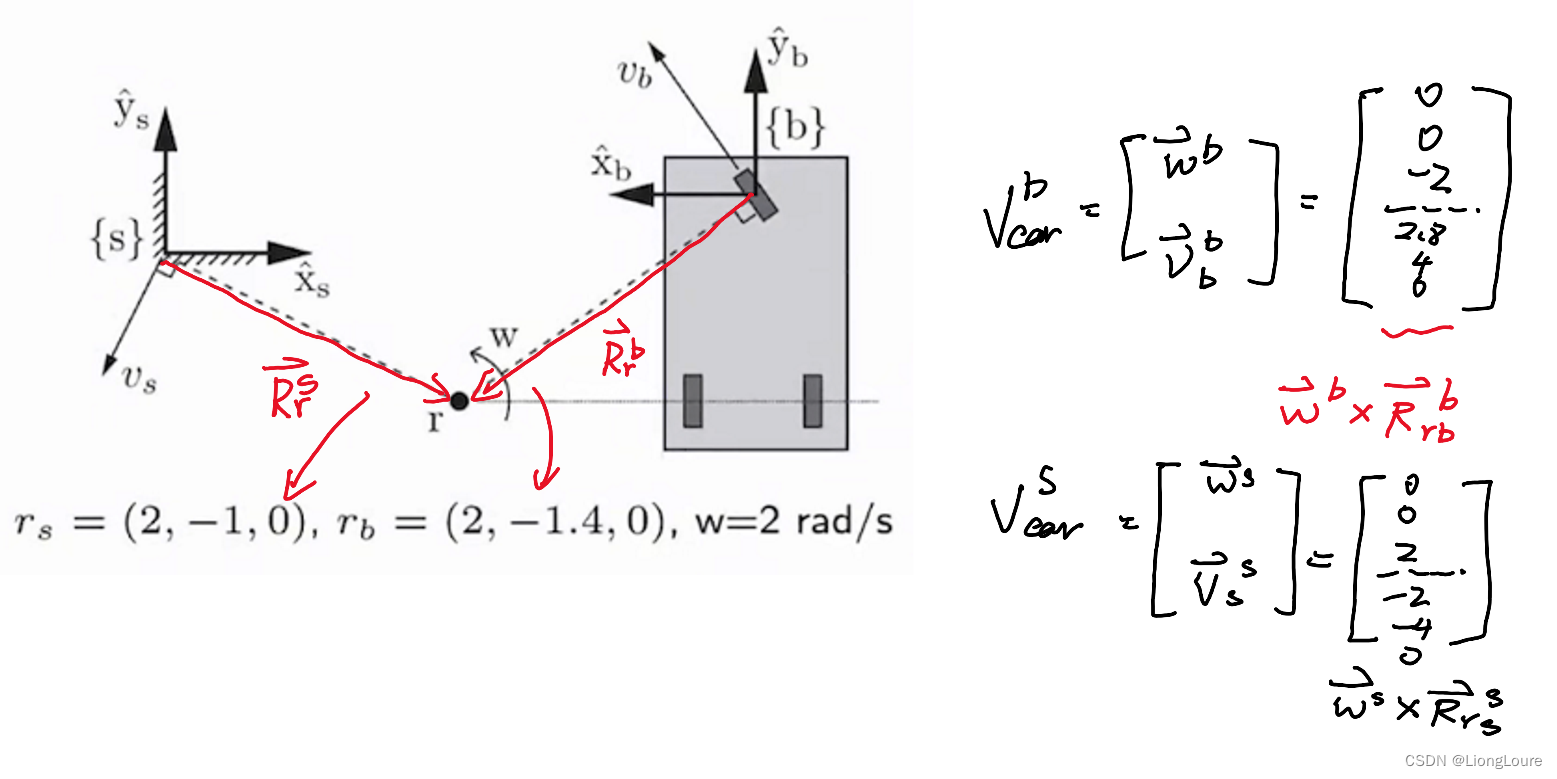
Example of Twist ,1:
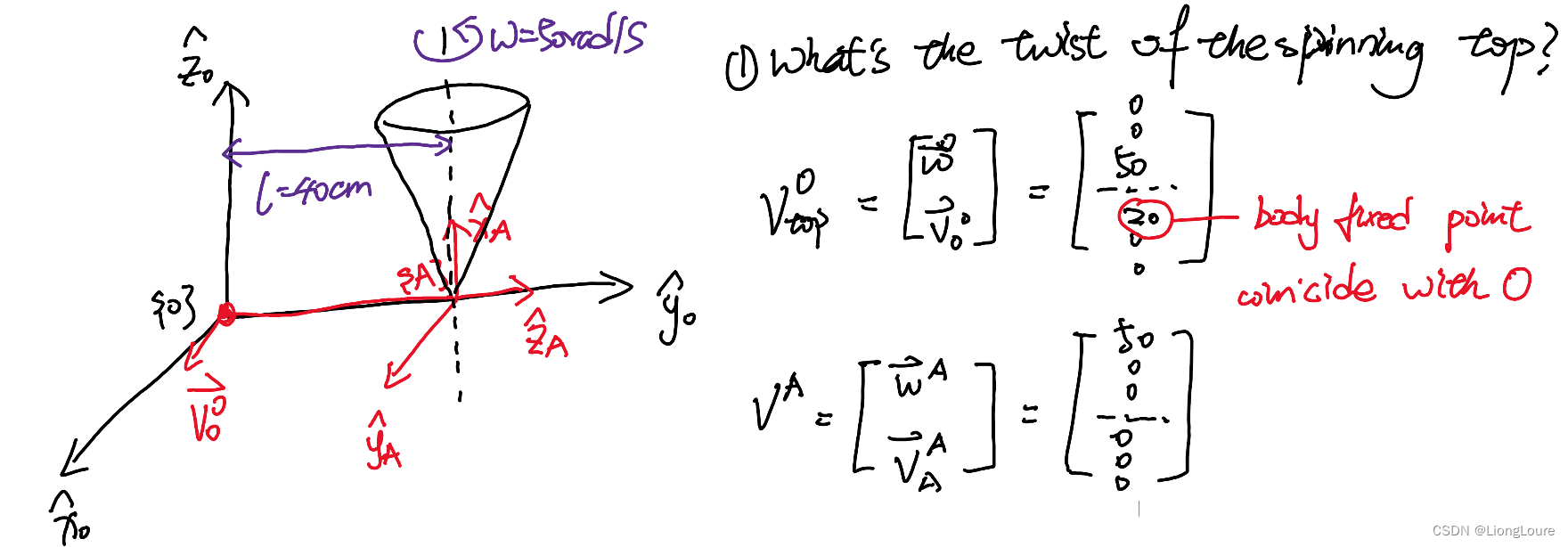
Example of Twist ,2:
2.3 Change Reference Frame for Twist
Given a twist V \mathcal{V} V , let V A \mathcal{V} ^A VA and V B \mathcal{V} ^B VB be their coordinates in frames { A } \left\{ A \right\} {A} and { B } \left\{ B \right\} {B} : V A = [ ω ⃗ A v ⃗ A ] , V B = [ ω ⃗ B v ⃗ B ] \mathcal{V} ^A=\left[ \begin{array}{c} \vec{\omega}^A\\ \vec{v}^A\\ \end{array} \right] ,\mathcal{V} ^B=\left[ \begin{array}{c} \vec{\omega}^B\\ \vec{v}^B\\ \end{array} \right] VA=[ωAvA],VB=[ωBvB]
- ω ⃗ A = [ Q B A ] ω ⃗ B \vec{\omega}^A=\left[ Q_{\mathrm{B}}^{A} \right] \vec{\omega}^B ωA=[QBA]ωB
- v ⃗ A A = v ⃗ B A + ω ⃗ A × R ⃗ B A A = [ Q B A ] v ⃗ B B + R ⃗ B A × ( [ Q B A ] ω ⃗ B ) = [ Q B A ] v ⃗ B B + R ⃗ ~ B A [ Q B A ] ω ⃗ B \vec{v}_{\mathrm{A}}^{A}=\vec{v}_{\mathrm{B}}^{A}+\vec{\omega}^A\times \vec{R}_{\mathrm{BA}}^{A}=\left[ Q_{\mathrm{B}}^{A} \right] \vec{v}_{\mathrm{B}}^{B}+\vec{R}_{\mathrm{B}}^{A}\times \left( \left[ Q_{\mathrm{B}}^{A} \right] \vec{\omega}^B \right) =\left[ Q_{\mathrm{B}}^{A} \right] \vec{v}_{\mathrm{B}}^{B}+\tilde{\vec{R}}_{\mathrm{B}}^{A}\left[ Q_{\mathrm{B}}^{A} \right] \vec{\omega}^B vAA=vBA+ωA×RBAA=[QBA]vBB+RBA×([QBA]ωB)=[QBA]vBB+R~BA[QBA]ωB
V A = [ ω ⃗ A v ⃗ A ] = [ [ Q B A ] 0 3 × 3 R ⃗ ~ B A [ Q B A ] [ Q B A ] ] 6 × 6 [ ω ⃗ B v ⃗ B ] = [ X B A ] V B \mathcal{V} ^A=\left[ \begin{array}{c} \vec{\omega}^A\\ \vec{v}^A\\ \end{array} \right] =\left[ \begin{matrix} \left[ Q_{\mathrm{B}}^{A} \right]& 0_{3\times 3}\\ \tilde{\vec{R}}_{\mathrm{B}}^{A}\left[ Q_{\mathrm{B}}^{A} \right]& \left[ Q_{\mathrm{B}}^{A} \right]\\ \end{matrix} \right] _{6\times 6}\left[ \begin{array}{c} \vec{\omega}^B\\ \vec{v}^B\\ \end{array} \right] =\left[ X_{\mathrm{B}}^{A} \right] \mathcal{V} ^B VA=[ωAvA]=[[QBA]R~BA[QBA]03×3[QBA]]6×6[ωBvB]=[XBA]VB
If configuration V B \mathcal{V} ^B VB in V A \mathcal{V} ^A VA is [ T B A ] = ( [ Q B A ] , R ⃗ B A ) \left[ T_{\mathrm{B}}^{A} \right] =\left( \left[ Q_{\mathrm{B}}^{A} \right] ,\vec{R}_{\mathrm{B}}^{A} \right) [TBA]=([QBA],RBA) , then : [ X B A ] = [ A d T ] = [ [ Q B A ] 0 R ⃗ ~ B A [ Q B A ] [ Q B A ] ] \left[ X_{\mathrm{B}}^{A} \right] =\left[ Ad_{\mathrm{T}} \right] =\left[ \begin{matrix} \left[ Q_{\mathrm{B}}^{A} \right]& 0\\ \tilde{\vec{R}}_{\mathrm{B}}^{A}\left[ Q_{\mathrm{B}}^{A} \right]& \left[ Q_{\mathrm{B}}^{A} \right]\\ \end{matrix} \right] [XBA]=[AdT]=[[QBA]R~BA[QBA]0[QBA]]——adjoint to T
3. Geometric Aspect of Twist: Screw Motion
v ⃗ = ∥ v ⃗ ∥ v ⃗ ^ , ω ⃗ = θ ˙ ω ⃗ ^ \vec{v}=\left\| \vec{v} \right\| \hat{\vec{v}},\vec{\omega}=\dot{\theta}\hat{\vec{\omega}} v=∥v∥v^,ω=θ˙ω^
3.1 Screw Motion : Definition
Screw Motion : Standard/
canonical/kə'nɒnɪk(ə)l/典型motion for rigid body motion
Rotating about an axis while also translating along the axis
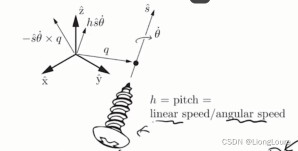
Represented by screw axis
{
R
⃗
q
,
s
^
,
h
}
\left\{ \vec{R}_q,\hat{s},h \right\}
{Rq,s^,h} and rotation speed
θ
˙
\dot{\theta}
θ˙ (derive the linear speed is
h
θ
˙
h\dot{\theta}
hθ˙)
- s ^ \hat{s} s^ : unit vector in the direction of the rotatin axis
- R ⃗ q \vec{R}_q Rq : any point on the rotation axis
- h h h : screw pitch which defines the ratio of the linear velocity along with the screw axis to the angular velocity about the screw axis
Theorem(Chasles) : Every rigid body motion can be realized by a screw motion
3.2 From Screw Motion to Twist
Consider a rigid body under a screw motion with screw axis
{
R
⃗
q
,
s
^
,
h
}
\left\{ \vec{R}_q,\hat{s},h \right\}
{Rq,s^,h} and rotation speed
θ
˙
\dot{\theta}
θ˙
Fix a reference frame
V
A
\mathcal{V} ^A
VA with origin
A
A
A
Find the Twist :
V
A
=
(
ω
⃗
A
,
v
⃗
A
A
)
=
(
s
^
A
θ
˙
,
v
⃗
q
A
+
ω
⃗
A
×
R
⃗
q
A
A
)
=
(
s
^
A
θ
˙
,
h
θ
˙
+
(
s
^
A
θ
˙
)
×
R
⃗
q
A
A
)
=
(
s
^
A
θ
˙
,
h
θ
˙
+
R
⃗
q
A
×
(
s
^
A
θ
˙
)
)
\mathcal{V} ^A=\left( \vec{\omega}^A,\vec{v}_{\mathrm{A}}^{A} \right) =\left( \hat{s}^A\dot{\theta},\vec{v}_{\mathrm{q}}^{A}+\vec{\omega}^A\times \vec{R}_{\mathrm{qA}}^{A} \right) =\left( \hat{s}^A\dot{\theta},h\dot{\theta}+\left( \hat{s}^A\dot{\theta} \right) \times \vec{R}_{\mathrm{qA}}^{A} \right) =\left( \hat{s}^A\dot{\theta},h\dot{\theta}+\vec{R}_{\mathrm{q}}^{A}\times \left( \hat{s}^A\dot{\theta} \right) \right)
VA=(ωA,vAA)=(s^Aθ˙,vqA+ωA×RqAA)=(s^Aθ˙,hθ˙+(s^Aθ˙)×RqAA)=(s^Aθ˙,hθ˙+RqA×(s^Aθ˙))
Result: given screw axis { R ⃗ q , s ^ , h } \left\{ \vec{R}_q,\hat{s},h \right\} {Rq,s^,h} with rotation speed θ ˙ \dot{\theta} θ˙ , the corresponding twist V A = ( ω ⃗ A , v ⃗ A A ) \mathcal{V} ^A=\left( \vec{\omega}^A,\vec{v}_{\mathrm{A}}^{A} \right) VA=(ωA,vAA) is given by :
ω ⃗ A = s ^ A θ ˙ , v ⃗ A A = h θ ˙ + R ⃗ q A × ( s ^ A θ ˙ ) \vec{\omega}^A=\hat{s}^A\dot{\theta},\vec{v}_{\mathrm{A}}^{A}=h\dot{\theta}+\vec{R}_{\mathrm{q}}^{A}\times \left( \hat{s}^A\dot{\theta} \right) ωA=s^Aθ˙,vAA=hθ˙+RqA×(s^Aθ˙)
The result holds as long as all the vectors and the twist are repersented in the same reference frame
3.3 From Twist to Screw Motion
The converse is true as well: given any twist V A = ( ω ⃗ A , v ⃗ A A ) \mathcal{V} ^A=\left( \vec{\omega}^A,\vec{v}_{\mathrm{A}}^{A} \right) VA=(ωA,vAA) we can always find the corresponding screw motion { R ⃗ q , s ^ , h } \left\{ \vec{R}_q,\hat{s},h \right\} {Rq,s^,h} and θ ˙ \dot{\theta} θ˙
- If
ω
⃗
=
0
\vec{\omega}=0
ω=0, then it is a pure translation(
h
=
∞
h=\infty
h=∞)
s ^ = v ⃗ ∥ v ⃗ ∥ , θ ˙ = ∥ v ⃗ ∥ , h = ∞ \hat{s}=\frac{\vec{v}}{\left\| \vec{v} \right\|},\dot{\theta}=\left\| \vec{v} \right\| ,h=\infty s^=∥v∥v,θ˙=∥v∥,h=∞, R ⃗ q \vec{R}_q Rq can be arbitrary - If
ω
⃗
≠
0
\vec{\omega}\ne 0
ω=0:
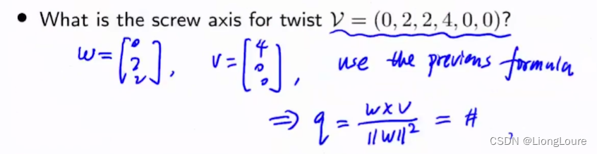
s ^ = ω ⃗ ∥ ω ⃗ ∥ , θ ˙ = ∥ ω ⃗ ∥ , R ⃗ q = ω ⃗ × v ⃗ ∥ ω ⃗ ∥ 2 , h = ω ⃗ T v ⃗ ∥ ω ⃗ ∥ \hat{s}=\frac{\vec{\omega}}{\left\| \vec{\omega} \right\|},\dot{\theta}=\left\| \vec{\omega} \right\| ,\vec{R}_{\mathrm{q}}=\frac{\vec{\omega}\times \vec{v}}{\left\| \vec{\omega} \right\| ^2},h=\frac{\vec{\omega}^{\mathrm{T}}\vec{v}}{\left\| \vec{\omega} \right\|} s^=∥ω∥ω,θ˙=∥ω∥,Rq=∥ω∥2ω×v,h=∥ω∥ωTv
You can pluf into the euqation above to very the result
Example: Screw Axin and Twist
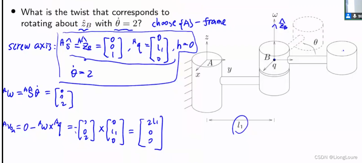
3.4 Screw Reoersentation of a Twist
- Recall : an angular velocity vector ω ⃗ \vec{\omega} ω can be viewed as θ ˙ ω ⃗ \dot{\theta}\vec{\omega} θ˙ω , where ω ⃗ \vec{\omega} ω is the unit ratation axis and θ ˙ \dot{\theta} θ˙ is the rate of rotation about that axis
Similarly, a twist (spatial velocity) V \mathcal{V} V can be interpreted in terms of a screw axis S ^ = { s ^ , h , R ⃗ q } \hat{\mathcal{S}}=\left\{ \hat{s},h,\vec{R}_q \right\} S^={s^,h,Rq} and a velocity θ ˙ \dot{\theta} θ˙ about the screw axis
Consider a rigid body motion along a screw axis
S
^
=
{
s
^
,
h
,
R
⃗
q
}
\hat{\mathcal{S}}=\left\{ \hat{s},h,\vec{R}_q \right\}
S^={s^,h,Rq} with speed
θ
˙
\dot{\theta}
θ˙. With slight abuse of notation, we will often write its twist as
V
=
θ
˙
S
^
\mathcal{V} =\dot{\theta}\hat{\mathcal{S}}
V=θ˙S^
In this notation, we think of S ^ \hat{\mathcal{S}} S^ as the twist associated with a unit speed motion along the screw axis { s ^ , h , R ⃗ q } \left\{ \hat{s},h,\vec{R}_q \right\} {s^,h,Rq}
4. Extra Note : Tutorial on Twist/spatial Velocity and Screw Axis
4.1 What is Spatial Velocity and Twist
- Twist/spatial velocity is the velocity of the whole rigid body, not velocity of a particular point
- Rigid body has inifinitely many points with different velocites
- All these velocites v ⃗ P i \vec{v}_{\mathrm{P}_{\mathrm{i}}} vPi are not independent, depend on the vector of its location and other parameters(common for the entire body), and can be experssed by same set of parameters(twist/spatial velocity is one such parameters)
- Assume
P
0
P_0
P0 is on the rotation axis/body-fixed, then any other body-fixed
pt. v ⃗ P i = v ⃗ P 0 + ω ⃗ × R ⃗ P 0 P i \vec{v}_{\mathrm{P}_{\mathrm{i}}}=\vec{v}_{\mathrm{P}_0}+\vec{\omega}\times \vec{R}_{\mathrm{P}_0\mathrm{P}_{\mathrm{i}}} vPi=vP0+ω×RP0Pi - What if we use
v
⃗
q
\vec{v}_{\mathrm{q}}
vq as the reference velocity, for arbitrary body-fixed
pt. q q q (may not be on rotation axis), we still have the same expression : v ⃗ P i = v ⃗ q + ω ⃗ × R ⃗ q P i \vec{v}_{\mathrm{P}_{\mathrm{i}}}=\vec{v}_{\mathrm{q}}+\vec{\omega}\times \vec{R}_{\mathrm{qP}_{\mathrm{i}}} vPi=vq+ω×RqPi
——use P 0 P_0 P0 as intermediate variable , q q q: body-fixed by above—— v ⃗ q = v ⃗ P 0 + ω ⃗ × R ⃗ P 0 P i = v ⃗ P i − ω ⃗ × R ⃗ q P i + ω ⃗ × R ⃗ P 0 P i \vec{v}_{\mathrm{q}}=\vec{v}_{P_0}+\vec{\omega}\times \vec{R}_{P_0\mathrm{P}_{\mathrm{i}}}=\vec{v}_{\mathrm{P}_{\mathrm{i}}}-\vec{\omega}\times \vec{R}_{\mathrm{qP}_{\mathrm{i}}}+\vec{\omega}\times \vec{R}_{P_0\mathrm{P}_{\mathrm{i}}} vq=vP0+ω×RP0Pi=vPi−ω×RqPi+ω×RP0Pi - Now let;s consider a frame
{
A
}
\left\{ A \right\}
{A} with origin
A
A
A
3.1 Assume { A } \left\{ A \right\} {A} body fixed, moves with the body (in this case , let point A A A is point q q q) v ⃗ P i = v ⃗ A + ω ⃗ × R ⃗ A P i \vec{v}_{\mathrm{P}_{\mathrm{i}}}=\vec{v}_{\mathrm{A}}+\vec{\omega}\times \vec{R}_{\mathrm{AP}_{\mathrm{i}}} vPi=vA+ω×RAPi in { A } \left\{ A \right\} {A} system : v ⃗ P i A = v ⃗ A A + ω ⃗ A × R ⃗ A P i A {\vec{v}_{\mathrm{P}_{\mathrm{i}}}}^A={\vec{v}_{\mathrm{A}}}^A+\vec{\omega}^A\times {\vec{R}_{\mathrm{AP}_{\mathrm{i}}}}^A vPiA=vAA+ωA×RAPiA
3.2 Assume { A } \left\{ A \right\} {A} NOT body-fixed ( { A } \left\{ A \right\} {A} does not move / moves in other way) , let q q q body fixes point such that R ⃗ q = R ⃗ A \vec{R}_{\mathrm{q}}=\vec{R}_{\mathrm{A}} Rq=RA , if we define v ⃗ A \vec{v}_{\mathrm{A}} vA as the velocity of the body-fixed point currently coincides wth A A A : v ⃗ P i = v ⃗ q ( t ) + ω ⃗ × R ⃗ q ( t ) P i = v ⃗ A + ω ⃗ × R ⃗ A P i \vec{v}_{\mathrm{P}_{\mathrm{i}}}=\vec{v}_{\mathrm{q}\left( t \right)}+\vec{\omega}\times \vec{R}_{\mathrm{q}\left( t \right) \mathrm{P}_{\mathrm{i}}}=\vec{v}_{\mathrm{A}}+\vec{\omega}\times \vec{R}_{\mathrm{AP}_{\mathrm{i}}} vPi=vq(t)+ω×Rq(t)Pi=vA+ω×RAPi
summary : Given twist V = ( ω ⃗ , v ⃗ A ) \mathcal{V} =\left( \vec{\omega}^{},\vec{v}_{\mathrm{A}}^{} \right) V=(ω,vA) , v ⃗ A \vec{v}_{\mathrm{A}}^{} vA velocity of body-fixed point currenting cioncides with A A A (reference poiny)
- For any body-fixed P i P_{\mathrm{i}} Pi: v ⃗ P i = v ⃗ A + ω ⃗ × R ⃗ A P i \vec{v}_{\mathrm{P}_{\mathrm{i}}}=\vec{v}_{\mathrm{A}}+\vec{\omega}\times \vec{R}_{\mathrm{AP}_{\mathrm{i}}} vPi=vA+ω×RAPi if A A A is origin of frame { A } \left\{ A \right\} {A} : v ⃗ P i A = v ⃗ A A + ω ⃗ A × R ⃗ A P i A {\vec{v}_{\mathrm{P}_{\mathrm{i}}}}^A={\vec{v}_{\mathrm{A}}}^A+\vec{\omega}^A\times {\vec{R}_{\mathrm{AP}_{\mathrm{i}}}}^A vPiA=vAA+ωA×RAPiA
- We can think the body is translating at velocity v ⃗ A \vec{v}_{\mathrm{A}} vA , while rotating at velocity ω ⃗ \vec{\omega} ω about axis passing through A A A
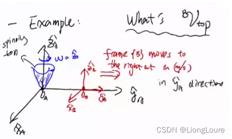

4.2 What is Screw Motion and Axis?
Screw motion : combined angular and linear motion
- motion driven by rotation
- parameters : { s ^ , h , R ⃗ q } \left\{ \hat{s},h,\vec{R}_q \right\} {s^,h,Rq} and θ ˙ \dot{\theta} θ˙: ( s ^ , R ⃗ q ) \left( \hat{s},\vec{R}_q \right) (s^,Rq) determeines the rotation axis; h h h linear speed / angular speed (due to thread on the screw - rotation induces linear motion)( h = 0 h=0 h=0-pure rotation, h = ∞ h=\infty h=∞-pure translation)
Over all { s ^ , h , R ⃗ q } \left\{ \hat{s},h,\vec{R}_q \right\} {s^,h,Rq} screw axis(rotation axis + pitch); θ ˙ \dot{\theta} θ˙ how fast screw rotates
- screw motion is a special rigid-body motion, so its has a twist
pitch a frame { A } \left\{ A \right\} {A} : ( s ^ , h , R ⃗ q ) + θ ˙ ⇒ [ ω ⃗ A v ⃗ A A ] , ω ⃗ A = θ ˙ s ^ , v ⃗ A A = ( h θ ˙ ) s ^ − ω ⃗ A × R ⃗ q \left( \hat{s},h,\vec{R}_q \right) +\dot{\theta}\Rightarrow \left[ \begin{array}{c} \vec{\omega}^A\\ \vec{v}_{\mathrm{A}}^{A}\\ \end{array} \right] , \vec{\omega}^A=\dot{\theta}\hat{s},\vec{v}_{\mathrm{A}}^{A}=\left( h\dot{\theta} \right) \hat{s}-\vec{\omega}^A\times \vec{R}_q (s^,h,Rq)+θ˙⇒[ωAvAA],ωA=θ˙s^,vAA=(hθ˙)s^−ωA×Rq use q q q sa the reference - Ant rigid-body motion can be viewed as screw motion. Given any twist V \mathcal{V} V , we can always find ( s ^ , h , R ⃗ q , θ ˙ ) \left( \hat{s},h,\vec{R}_q,\dot{\theta} \right) (s^,h,Rq,θ˙)
- We know
V
=
S
c
r
e
w
T
o
T
w
i
s
t
(
s
^
,
h
,
R
⃗
q
,
1
)
θ
˙
=
θ
˙
S
\mathcal{V} =ScrewToTwist\left( \hat{s},h,\vec{R}_q,1 \right) \dot{\theta}=\dot{\theta}\mathcal{S}
V=ScrewToTwist(s^,h,Rq,1)θ˙=θ˙S while
S
\mathcal{S}
S the twist corresponds to screw motion
(
s
^
,
h
,
R
⃗
q
)
,
θ
˙
=
1
\left( \hat{s},h,\vec{R}_q \right) ,\dot{\theta}=1
(s^,h,Rq),θ˙=1
eg. ω ⃗ = θ ˙ ω ^ \vec{\omega}=\dot{\theta}\hat{\omega} ω=θ˙ω^ , ω ^ \hat{\omega} ω^ : rotation axis or angular velocity when rotates about ω ^ \hat{\omega} ω^ at θ ˙ = 1 \dot{\theta}=1 θ˙=1
Summarize : Given any rigid-body motion V = [ ω ⃗ v ⃗ A ] \mathcal{V} =\left[ \begin{array}{c} \vec{\omega}\\ \vec{v}_{\mathrm{A}}^{}\\ \end{array} \right] V=[ωvA] , with angular direction ω ^ \hat{\omega} ω^ linear motion direction v ^ \hat{v} v^ , knows screw axis direction S ^ \hat{\mathcal{S}} S^—— V = θ ˙ S ^ \mathcal{V} =\dot{\theta}\hat{\mathcal{S}} V=θ˙S^