brief

InferCNV is used to explore tumor single cell RNA-Seq data to identify evidence for somatic large-scale chromosomal copy number alterations, such as gains or deletions of entire chromosomes or large segments of chromosomes. This is done by exploring expression intensity of genes across positions of tumor genome in comparison to a set of reference ‘normal’ cells.

通过和‘normal’ cell的基因组位置相比，识别癌细胞基因组对应位置上发生的变化。

染色体畸变的 类型很多的，有结构上的（片段插入，片段缺失，重组，染色体断裂等等），有数量上的（染色体加倍，非整倍体，基因片段gain or lost）等等。

infercnv利用单细胞数据识别这些畸变，让我觉得很不可思议（测序深度，以及3‘或者5’端建库方法，可变剪接等等都会导致结果不可信）。不过很多的文章都在用它解析单细胞数据，我也不能仅仅停留在diss它的位置上，开学吧。

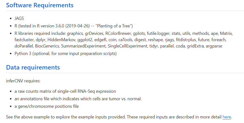
安装

# ubuntu 20
# https://sourceforge.net/projects/mcmc-jags/files/JAGS/4.x/Source/
wget https://sourceforge.net/projects/mcmc-jags/files/JAGS/4.x/Source/JAGS-4.3.2.tar.gz
tar -zxvf JAGS-4.3.2.tar.gz
cd JAGS-4.3.0
./configure --libdir=/usr/local/lib64
make
make install

if (!requireNamespace("BiocManager", quietly = TRUE))
     install.packages("BiocManager")
BiocManager::install("infercnv")

安装成功的验证

R
library(infercnv)

infercnv_obj = CreateInfercnvObject(raw_counts_matrix=system.file("extdata", "oligodendroglioma_expression_downsampled.counts.matrix.gz", package = "infercnv"),
                                    annotations_file=system.file("extdata", "oligodendroglioma_annotations_downsampled.txt", package = "infercnv"),
                                    delim="\t",
                                    gene_order_file=system.file("extdata", "gencode_downsampled.EXAMPLE_ONLY_DONT_REUSE.txt", package = "infercnv"),
                                    ref_group_names=c("Microglia/Macrophage","Oligodendrocytes (non-malignant)")) 

infercnv_obj = infercnv::run(infercnv_obj,
                             cutoff=1, # cutoff=1 works well for Smart-seq2, and cutoff=0.1 works well for 10x Genomics
                             out_dir=tempfile(), 
                             cluster_by_groups=TRUE, 
                             denoise=TRUE,
                             HMM=TRUE)

使用体验

输入文件制作

# 内置的raw counts文件
rwa_counts <- read.table(gzfile("/public/home/djs/miniconda3/envs/R4/lib/R/library/infercnv/extdata/oligodendroglioma_expression_downsampled.counts.matrix.gz","r"),sep="\t",header=T)

行是基因，列是细胞

# 内置的 cell annotation file
annotation_file <- read.table("/public/home/djs/miniconda3/envs/R4/lib/R/library/infercnv/extdata/oligodendroglioma_annotations_downsampled.txt",sep="\t",header=T)

文件分为两列，第一列记录细胞名称，第二列记录细胞注释类型，比如normal，malignant。

# 内置的基因坐标文件
gene_order <- read.table("/public/home/djs/miniconda3/envs/R4/lib/R/library/infercnv/extdata/gencode_downsampled.EXAMPLE_ONLY_DONT_REUSE.txt",sep="\t",header=T)

文件分为四列，第一列记录基因名称，第二列记录基因在哪条染色体上，以及第三四列记录染色体上的起始终止位点。

---

开始制作输入文件…

# 得到最容易得到的表达矩阵
sce <- readRDS("immune.integrated.annotation.rds") # seurat对象
dim(sce@meta.data)
# [1] 57970    13
raw_counts <- as.matrix(sce@assays$RNA@data) # 得到全部细胞的表达矩阵 
# 我这个数据集大约58000个细胞，软件运行的很慢而且再服务器上出图会报错，我打算取一些子集演示一下
# 只取上皮细胞
sce1 <- subset(sce,subset = singleR == "Epithelial_cells")
dim(sce1@meta.data)
# [1] 14938    13
raw_counts <- as.matrix(sce1@assays$RNA@data)
raw_counts[1:5,1:5] # 此时行是基因，列是细胞

# 现在 需要得到细胞的注释信息，一列是细胞名称，一列是细胞类型注释。
head(sce1@meta.data)
celltype <- sce1@meta.data[,"singleR"]
cellname <- rownames(sce1@meta.data)
annotation_file <- as.data.frame(cbind(cellname,celltype))

write.table(annotation_file,file="annotation_file.txt",sep="\t",row.names=F,col.names=F)

# 最后是基因在染色体上的坐标文件，这个因为不同的基因组注释文件以及版本可能有些不一样，应该是bug最多的一个文件了
# 归根揭底其实就是解析GTF/GFF文件
# https://www.gencodegenes.org/pages/data_format.html 这是gencode官网提供的信息，最后还贴心的附上了提取信息的code
cat ~/software/STAR-2.7.7a/genome_gtf/gencode.v40.annotation.gtf |  \
 awk '{if($3=="gene" && $0~"level (1|2);") {print $10,$14,$12,$1,$4,$5,$7}}'  | \
 sed 's/[";]//g' |sed 's/ /\t/g' | \
 sed  '1i ENSG_id \t gene_symbl \t gene_type \t chr\t start \t end'  > infercnv_gene_order.file.tsv

# 拿到这个这个文件后，再去R里面抓取表达矩阵出现的那些基因
gene_order <- read.table("/public/home/djs/reference/infercnv_gene_order.file.tsv",header=T,sep="\t")
gene_order <- gene_order[!duplicated(gene_order$ENSG_id),]
gene_order[1:5,]

# 很烦人，有些基因的名字不在注释文件中，看了一下大部分基因名字都是因为有后缀
length(rownames(raw_counts))
# [1] 25870
table(rownames(raw_counts) %in% gene_order$ENSG_id)
# FALSE  TRUE
# 6308 19562

# 算了，还是修改表达矩阵吧，也就是把那些没在gene_order中的基因丢了
raw_counts <- raw_counts[which(rownames(raw_counts) %in% gene_order$ENSG_id),]
dim(raw_counts)
# [1] 19562 14938

gene_order_file <- gene_order[which(gene_order$ENSG_id %in% rownames(raw_counts)),c(1,3,4,5)]
write.table(raw_counts,file="raw_counts_file.txt",sep="\t",row.names=T)  # 需要把基因作为行名写入文件
write.table(gene_order_file,file="gene_order_file.txt",sep="\t",row.names=F,col.names=F) # 行列名不需要写入

运行试试吧

# create the infercnv object
infercnv_obj = CreateInfercnvObject(raw_counts_matrix="raw_counts_file.txt",
                                    annotations_file="annotation_file.txt",
                                    delim="\t",
                                    gene_order_file="gene_order_file.txt",
                                    ref_group_names=NULL)
                                    
# perform infercnv operations to reveal cnv signal
infercnv_obj = infercnv::run(infercnv_obj,
                             cutoff=0.1,  # use 1 for smart-seq, 0.1 for 10x-genomics
                             out_dir="output_dir",  # dir is auto-created for storing outputs
                             cluster_by_groups=T,   # cluster
                             denoise=T,
                             HMM=T
                             )

• ref_group_names参数的使用：
  Note, if you do not have reference cells, you can set ref_group_names=NULL, in which case the average signal across all cells will be used to define the baseline. This can work well when there are sufficient differences among the cells included
  也可以设置为 ref_group_names=c("NK_cell"))

• 需要注意的是cutoff 值，这是噪音过滤参数：
  The cutoff value determines which genes will be used for the infercnv analysis. Genes with a mean number of counts across cells will be excluded. For smart-seq (full-length transcript sequencing, typically using cell plate assays rather than droplets), a value of 1 works well. For 10x (and potentially other 3’-end sequencing and droplet assays, where the count matrix tends to be more sparse), a value of 0.1 is found to generally work well.

• inferCNV de-noising filters是为了干什么？还有其他方法吗？
  These de-noising filter options are available for manipulating the residual expression intensities with the goal of reducing the noise (residual signal in the normal cells) while retaining the signal in tumor cells that could be interpreted as supporting CNV.

  把normal 细胞的表达信号当作背景信号，其他细胞的表达信号减去背景信号，也就是获取偏离normal 的信号，认为他们是gain or loss CNV。

# 手动指定背景信号值
# A specific threshold deviation from the mean can be set using the 'noise_filter' attribute
 infercnv_obj = infercnv::run(infercnv_obj,
                             cutoff=1, # cutoff=1 works well for Smart-seq2, and cutoff=0.1 works well for 10x Genomics
                             out_dir=out_dir, 
                             cluster_by_groups=T, 
                             plot_steps=F,
                             denoise=T,
                             noise_filter=0.1   ## hard thresholds
                             )

# 更具偏离标准差的距离设定阈值
By default, the hard cutoffs for denoising are computed based on the standard deviation of the residual normal expression values. This thresholding can be adjusted using the 'sd_amplifier' setting.
infercnv_obj = infercnv::run(infercnv_obj,
                             cutoff=1, # cutoff=1 works well for Smart-seq2, and cutoff=0.1 works well for 10x Genomics
                             out_dir=out_dir, 
                             cluster_by_groups=T, 
                             plot_steps=F,
                             denoise=T,
                             sd_amplifier=1.5  ## set dynamic thresholding based on the standard deviation value.
                             )

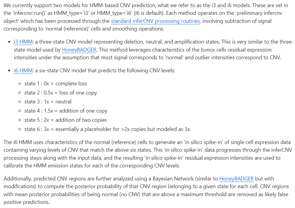
• 预测CNV的方法以及结果
  

• 另一个参数细节：
  By setting infercnv::run(analysis_mode=‘subclusters’), inferCNV will attempt to partition cells into groups having consistent patterns of CNV. CNV prediction (via HMM) would then be performed at the level of the subclusters rather than whole samples.
  （The methods available for defining tumor subclusters will continue to be expanded. We’ve currently had best success with using hierarchical clustering based methods.）

结果部分

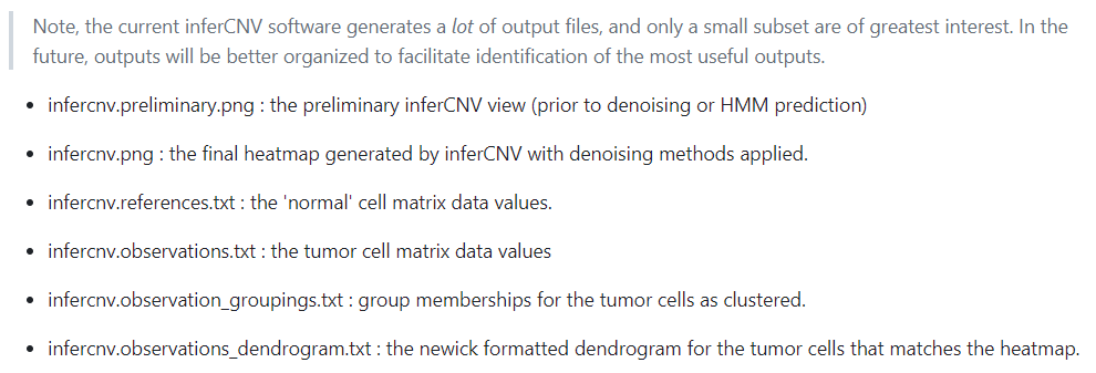
出现最后的 making the final infercnv heatmap才是正常结束，运行时间大应该是14938个细胞13：00-19：00

• 了解一下都是些什么结果然后如何结合seurat对象作图
  

• 判定恶性细胞
  参考文章：
  https://cloud.tencent.com/developer/inventory/7049/article/1737138
  https://cloud.tencent.com/developer/inventory/7049/article/1737241

# 读取infercnv.observations.txt文件来计算CNV score

cnv_table <- read.table("plot_out/inferCNV_output2/infercnv.observations.txt", header=T)
# Score cells based on their CNV scores 
# Replicate the table 
cnv_score_table <- as.matrix(cnv_table)
cnv_score_mat <- as.matrix(cnv_table)
# Scoring
# CNV的5分类系统
cnv_score_table[cnv_score_mat > 0 & cnv_score_mat < 0.3] <- "A" #complete loss. 2pts
cnv_score_table[cnv_score_mat >= 0.3 & cnv_score_mat < 0.7] <- "B" #loss of one copy. 1pts
cnv_score_table[cnv_score_mat >= 0.7 & cnv_score_mat < 1.3] <- "C" #Neutral. 0pts
cnv_score_table[cnv_score_mat >= 1.3 & cnv_score_mat <= 1.5] <- "D" #addition of one copy. 1pts
cnv_score_table[cnv_score_mat > 1.5 & cnv_score_mat <= 2] <- "E" #addition of two copies. 2pts
cnv_score_table[cnv_score_mat > 2] <- "F" #addition of more than two copies. 2pts

# Check
table(cnv_score_table[,1])
# Replace with score 
cnv_score_table_pts <- cnv_table
rm(cnv_score_mat)
#  把5分类调整为 3分类系统
cnv_score_table_pts[cnv_score_table == "A"] <- 2
cnv_score_table_pts[cnv_score_table == "B"] <- 1
cnv_score_table_pts[cnv_score_table == "C"] <- 0
cnv_score_table_pts[cnv_score_table == "D"] <- 1
cnv_score_table_pts[cnv_score_table == "E"] <- 2
cnv_score_table_pts[cnv_score_table == "F"] <- 2

# Scores are stored in “cnv_score_table_pts”. Use colSums to add up scores for each cell and store as vector 
cell_scores_CNV <- as.data.frame(colSums(cnv_score_table_pts))
colnames(cell_scores_CNV) <- "cnv_score"
head(cell_scores_CNV)
write.csv(x = cell_scores_CNV, file = "cnv_scores.csv") # 根据这个文件给每个细胞打分或者划高低中等分类然后比较或者可视化

我自己的数据集中每个基因的 CNV score都“适中”，大概是因为我没有提供“reference normal cell”，所以上述代码就不搞了。
（打完分就可以得到cell barcode，这些cell barcode 结合 seurat object 就可以可视化到UMAP等图中了）

---

算法思想细节
The detailed steps of the inferCNV algorithm involve the following:

• filtering genes: those genes found expressed in fewer than ‘min_cells_per_gene’ are removed from the counts matrix.
  把低表达基因基因去除

• normalization for sequencing depth (total sum normalization): read counts per cell are scaled to sum to the median total read count across cells. Instead of a metric such as counts per million (cpm), values are counts per median sum.
  这里的normalization方法就很特殊 = （reads / total reads）* median of all sum reads from all cells

• log transformation: individual matrix values (x) are transformed to log(x+1)
  normalization 后 再log transformation

• center by normal gene expression: the mean value for each gene across normal (reference) cells is subtracted from all cells for corresponding genes. Since this subtraction is performed in log space, this is effectively resulting in log-fold-change values relative to the mean of the normal cells.
  每个基因的scale

• thresholding dynamic range for log-fold-change values. Any values with abs(log(x+1)) exceeding ‘max_centered_threshold’ (default=3) are capped at that value.

• chromosome-level smoothing: for each cell, genes ordered along each chromosome have expression intensities smoothed using a weighted running average. By default, this is a window of 101 genes with a pyramidinal weighting scheme.

• centering cells: each cell is centered with its median expression intensity at zero under the assumption that most genes are not in CNV regions.

• adjustment relative to normal cells: The mean of the normals is once again subtracted from the tumor cells. This further compensates for differences that accrued after the smoothing process.

• the log transformation is reverted. This makes the evidence for amplification or deletion more symmetrical around the mean. (note, with loss or gain of one copy, corresponding values 0.5 and 1.5 are not symmetrical in log space. Instead, 0.5 and 2 are symmetrical in log space. Hence, we invert the log transformation to better reflect symmetry in gains and losses).

others