这里写目录标题
- UPA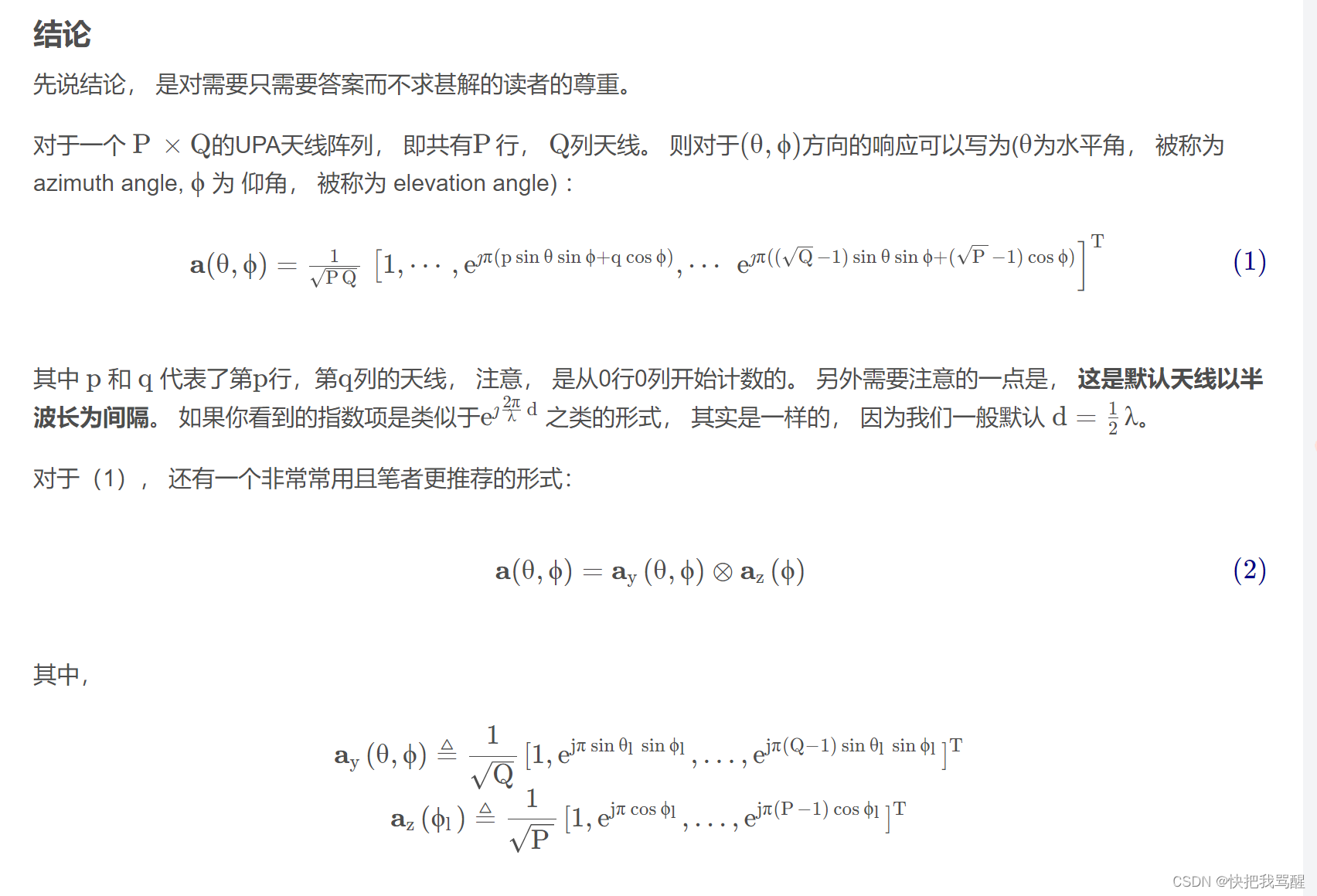
- 写在前面
- Channel Estimation for Extremely Large-Scale Massive MIMO:Far-Field, Near-Field, or Hybrid-Field?
- Far Field model
- Near Field model
UPA
写在前面
Dai Linglong老师的简介网站
Channel Estimation for Extremely Large-Scale Massive MIMO:Far-Field, Near-Field, or Hybrid-Field?
 近场的方向向量,把里边每一项做泰勒展开,如果把高阶项近似为0,则为远场。近场是保留了二阶小量,然后远场是只保留一阶小量。
信道估计: 已知发射端发射导频和接收端的接收导频信号估计信道。
N
N
N BS处天线数
D
D
D 天线孔径
λ
\lambda
λ 天线波长
瑞利距离
Z
Z
Z:
Z
=
2
D
2
/
λ
Z = 2D^2/\lambda
Z=2D2/λ
Far Field model
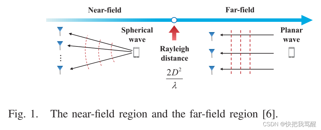
- Far-Field Channel Model: As shown in Fig. 1, when the distance between the BS and the scatter is larger than the Rayleigh distance, the far-field channel h far-field \mathbf{h}_{\text {far-field }} hfar-field is modeled under the planar wave assumption, which can be represented by
h far-field = N L ∑ l = 1 L α l a ( θ l ) (3) \mathbf{h}_{\text {far-field }}=\sqrt{\frac{N}{L}} \sum_{l=1}^{L} \alpha_{l} \mathbf{a}\left(\theta_{l}\right) \tag{3} hfar-field =LNl=1∑Lαla(θl)(3)
where L L L represents the number of path components (corresponding to effective scatters) between the BS and the user, α l \alpha_{l} αl and θ l \theta_{l} θl represent the gain and angle for the l l lth path, respectively. a ( θ l ) \left(\theta_{l}\right) (θl) represents the far-field array steering vector based on the planar wave assumption, which can represented by`
a ( θ l ) = 1 N [ 1 , e − j π θ l , … , e − j ( N − 1 ) π θ l ] H (4) \mathbf{a}\left(\theta_{l}\right)=\frac{1}{\sqrt{N}}\left[1, e^{-j \pi \theta_{l}}, \ldots, e^{-j(N-1) \pi \theta_{l}}\right]^{H} \tag{4} a(θl)=N1[1,e−jπθl,…,e−j(N−1)πθl]H(4)
It is noted that θ l = 2 d λ cos ( ϕ l ) \theta_{l}=2 \frac{d}{\lambda} \cos \left(\phi_{l}\right) θl=2λdcos(ϕl) , where d = λ 2 d=\frac{\lambda}{2} d=2λ is the antenna spacing, and ϕ l ∈ ( 0 , π ) \phi_{l} \in(0, \pi) ϕl∈(0,π) is the practical physical angle.
In order to reduce the pilot overhead for the channel estimation, the above non-sparse channel h far-field \mathbf{h}_{\text {far-field }} hfar-field can be represented by the sparse angle-domain channel h far-field A \mathbf{h}_{\text {far-field }}^{A} hfar-field A with the DFT matrix F \mathbf{F} F as follows
h far-field = F h far-field A (5) \mathbf{h}_{\text {far-field }}=\mathbf{F} \mathbf{h}_{\text {far-field }}^{A} \tag{5} hfar-field =Fhfar-field A(5)
where F = [ a ( θ 1 ) , … , a ( θ N ) ] \mathbf{F}=\left[\mathbf{a}\left(\theta_{1}\right), \ldots, \mathbf{a}\left(\theta_{N}\right)\right] F=[a(θ1),…,a(θN)] is a N N N \times N N N unitary matrix, where the columns are orthogonal to each other, and θ n = 2 n − N − 1 N \theta_{n}= \frac{2 n-N-1}{N} θn=N2n−N−1 with n = 1 , 2 , … , N n=1,2, \ldots, N n=1,2,…,N . Since there are limited scatters in communication environments, the angle-domain channel h far-field A \mathbf{h}_{\text {far-field }}^{A} hfar-field A is usually sparse. Based on this sparsity, some CS algorithms can be used to estimate this high-dimensional channel with low pilot overhead [3]-[5].
Near Field model
除了上述远场信道模型之外,最近在[6]中提出了近场信道模型。如图1所示,当基站与散射体之间的距离小于瑞利距离时,近场信道在球面波假设下建模,可以表示为
h near-field = N L ∑ l = 1 L α l b ( θ l , r l ) (6) \mathbf{h}_{\text {near-field }}=\sqrt{\frac{N}{L}} \sum_{l=1}^{L} \alpha_{l} \mathbf{b}\left(\theta_{l}, r_{l}\right) \tag{6} hnear-field =LNl=1∑Lαlb(θl,rl)(6)
与远场信道模型(3)相比,基于球面波假设推导了近场信道模型的阵列导向矢量 b ( θ l , r l ) \mathbf{b}\left(\theta_{l}, r_{l}\right) b(θl,rl),可以表示为[6]
b ( θ l , r l ) = 1 N [ e − j 2 π λ ( r l ( 1 ) − r l ) , … , e − j 2 π λ ( r l ( N ) − r l ) ] H (7) \mathbf{b}\left(\theta_{l}, r_{l}\right)=\frac{1}{\sqrt{N}}\left[e^{-j \frac{2 \pi}{\lambda}\left(r_{l}^{(1)}-r_{l}\right)}, \ldots, e^{-j \frac{2 \pi}{\lambda}\left(r_{l}^{(N)}-r_{l}\right)}\right]^{H} \tag{7} b(θl,rl)=N1[e−jλ2π(rl(1)−rl),…,e−jλ2π(rl(N)−rl)]H(7)
where r l r_{l} rl represents the distance from the l l l th scatter to the center of the antenna array, r l ( n ) = r l 2 + δ n 2 d 2 − 2 r l δ n d θ l r_{l}^{(n)}=\sqrt{r_{l}^{2}+\delta_{n}^{2} d^{2}-2 r_{l} \delta_{n} d \theta_{l}} rl(n)=rl2+δn2d2−2rlδndθl represents the distance from the l l l th scatter to the n n n th BS antenna, and δ n = 2 n − N − 1 2 \delta_{n}=\frac{2 n-N-1}{2} δn=22n−N−1 with n = 1 , 2 , … , N n=1,2, \ldots, N n=1,2,…,N .
Since the DFT matrix in (5) associated with the angle domain only matches the array steering vector in the far-field, the near-field channel in (6) will cause serious energy spread in angle domain. In order to explore the sparsity of the near-field channel, a polar-domain transform matrix W \mathbf{W} W was proposed in [6], which can be represented by (为了探索近场信道的稀疏性,极化域变换矩阵 W \mathbf{W} W)
W = [ b ( θ 1 , r 1 1 ) , … , b ( θ 1 , r 1 S 1 ) , … , b ( θ N , r N 1 ) , … , b ( θ N , r N S N ) ] (8) \begin{array}{r} \mathbf{W}=\left[\mathbf{b}\left(\theta_{1}, r_{1}^{1}\right), \ldots, \mathbf{b}\left(\theta_{1}, r_{1}^{S_{1}}\right), \ldots,\right. \\ \left.\quad \mathbf{b}\left(\theta_{N}, r_{N}^{1}\right), \ldots, \mathbf{b}\left(\theta_{N}, r_{N}^{S_{N}}\right)\right] \end{array} \tag{8} W=[b(θ1,r11),…,b(θ1,r1S1),…,b(θN,rN1),…,b(θN,rNSN)](8)
where each column of W \mathbf{W} W is a near-field array steering vector with the sampled angle θ n \theta_{n} θn and distance r n s n r_{n}^{s_{n}} rnsn , with s n = 1 , 2 , … , S n s_{n}= 1,2, \ldots, S_{n} sn=1,2,…,Sn, S n S_{n} Sn represents the number of sampled distances at the sampled angle θ n \theta_{n} θn . Thus, the number of all sampled grids can be represented by S = ∑ n = 1 N S n S=\sum_{n=1}^{N} S_{n} S=∑n=1NSn . Based on this polar-domain transform matrix W \mathbf{W} W , the near-field channel can be represented by
近场把信道变换到极化域(在极化域中信道是稀疏的)
h near-field = W h near-field P (9) \mathbf{h}_{\text {near-field }}=\mathbf{W} \mathbf{h}_{\text {near-field }}^{P} \tag{9} hnear-field =Whnear-field P(9)
where h near-field P \mathbf{h}_{\text {near-field }}^{P} hnear-field P is the S × 1 S \times 1 S×1 polar-domain channel. Similar to the far-field channel in the angle domain, h near-field P \mathbf{h}_{\text {near-field }}^{P} hnear-field P also shows a certain sparsity. The corresponding polar-domain based CS algorithm was further proposed to reduce the pilot overhead for the near-field channel estimation [6]. However, since the polar transform matrix W \mathbf{W} W is generated from the joint angle and distance space, its dimension is large, and the columns orthogonality is relatively poor compared with the DFT matrix. Thus, the far-field channel in the polar domain may cause more serious energy leakage than that in the angle domain.
极化域的远场通道可能比角域的远场通道造成更严重的能量泄漏。
在上述所有现有工作中,通信环境中的所有散射都假设位于远场或近场区域。在实际的XL-MIMO通信环境中,更有可能一些散射位于远场区域,而另一些则可能位于近场区域。然而,这种混合场通信环境无法通过现有的远场或近场信道模型来精确建模,因此现有的远场和近场信道估计方案不能直接用于精确估计混合场XL- MIMO 信道。