本期内容
读取多个盐度文件;

拼接数据

在画盐度的季节分布图
Part01.
使用数据

IAP 网格盐度数据集
数据详细介绍:
见文件附件:
pages/file/dl?fid=378649712527544320
全球温盐格点数据.pdf
IAP_Global_ocean_gridded_product.pdf
全球温盐格点数据.pdf
IAP_Global_ocean_gridded_product.pdf
Part02.
读取nc的语句
import xarray as xr
f1 = xr.open_dataset(filelist[1])
print(f1)
Dimensions:    (lat: 180, lon: 360, time: 1, depth_std: 41)

Coordinates:
  * lat        (lat) float32 -89.5 -88.5 -87.5 -86.5 ... 86.5 87.5 88.5 89.5
  * lon        (lon) float32 1.0 2.0 3.0 4.0 5.0 ... 357.0 358.0 359.0 360.0
  * time       (time) float32 2.02e+05
  * depth_std  (depth_std) float32 1.0 5.0 10.0 20.0 ... 1.7e+03 1.8e+03 2e+03
Data variables:
    salinity   (lat, lon, depth_std) float32 ...
Attributes:
    Title:           IAP 3-Dimentional Subsurface Salinity Dataset Using IAP ...
    StartYear:       2020
    StartMonth:      2
    StartDay:        1
    EndYear:         2020
    EndMonth:        2
    EndDay:          30
    Period:          1
    GridProjection:  Mercator, gridded
    GridPoints:      360x180
    Creator:         Lijing Cheng From IAP,CAS,P.R.China
    Reference:       ****. Website: http://159.226.119.60/cheng/
Part03.
盐度季节的求法
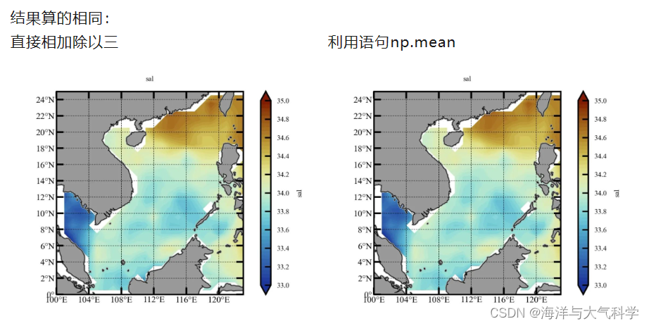
2:春季3-4-5
直接相加除以三
sal_spr = (sal_all[2, :, :]+sal_all[3, :, :]+sal_all[4, :, :])/3
利用语句np.mean
sal_spr_new = np.mean(sal_all[2:5,:,:], axis=0)
结果算的相同:
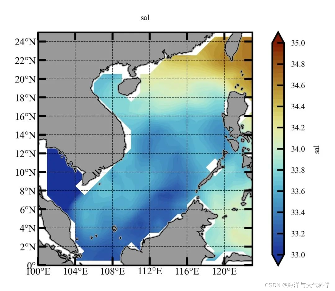
全年平均:
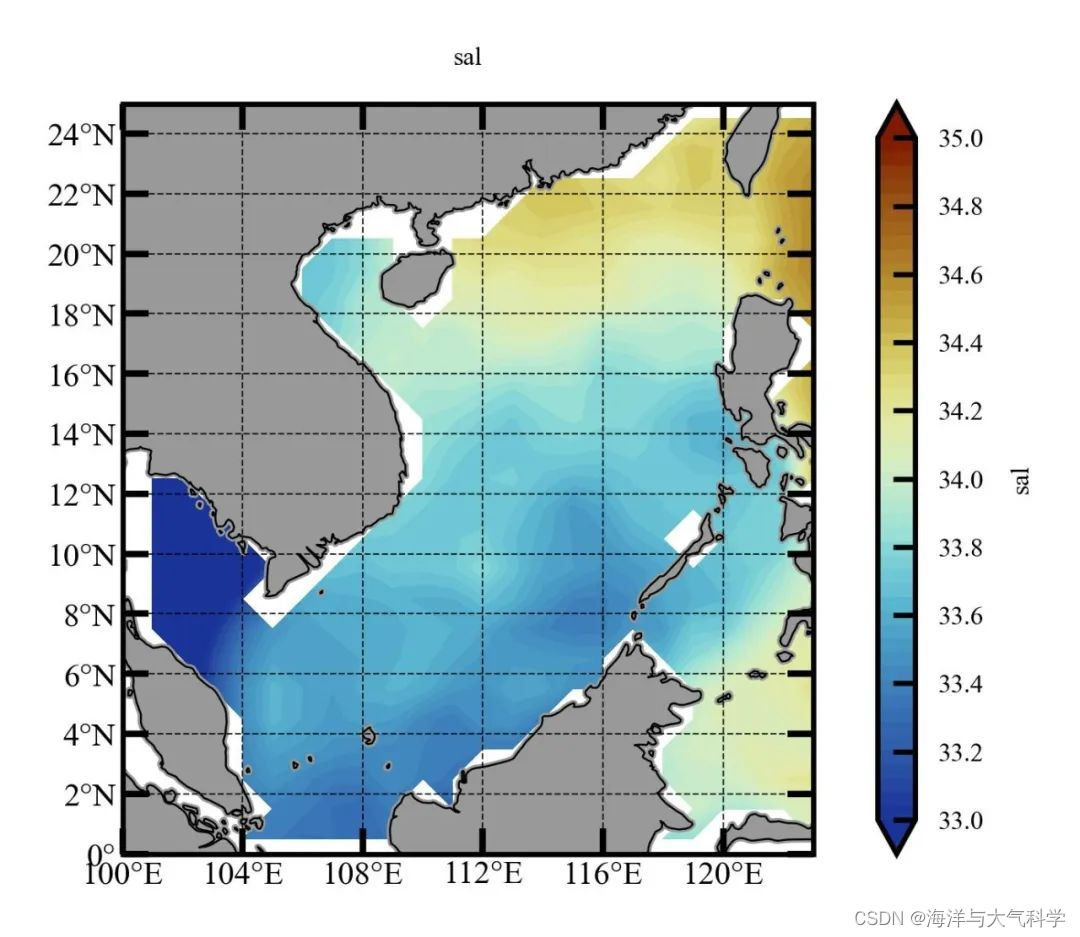
春季:
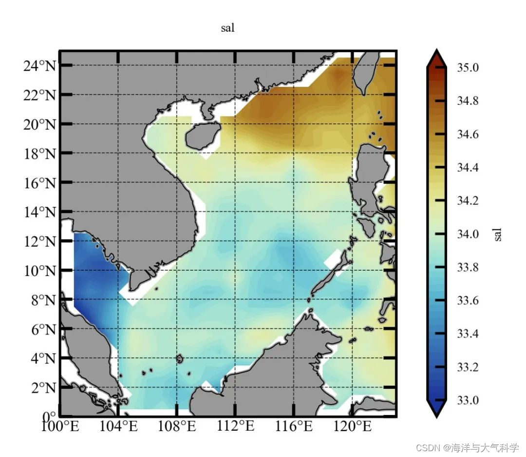
夏季:
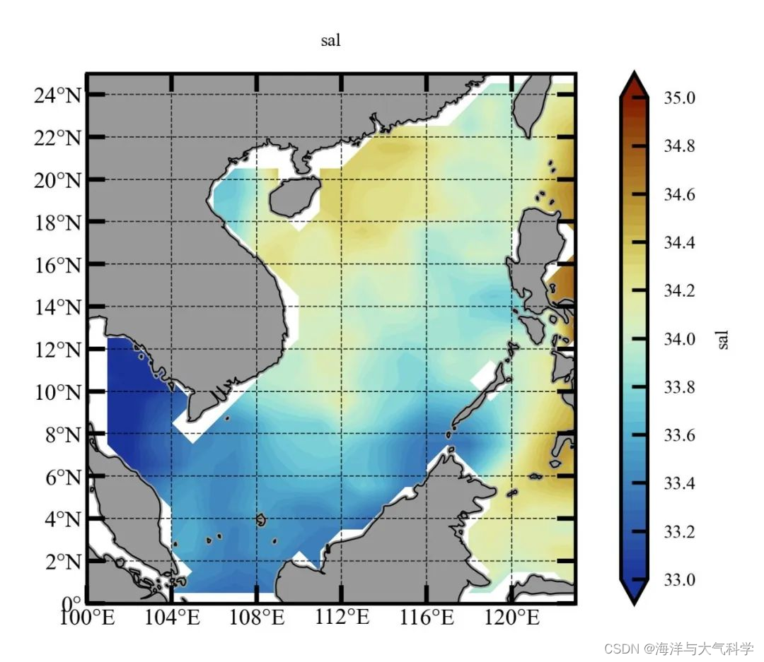
秋季:
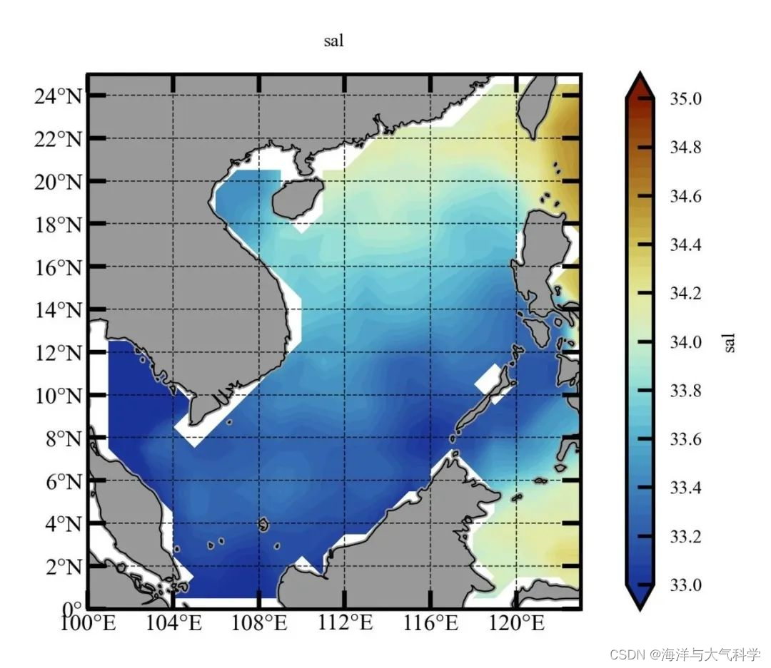
冬季:
往期推荐
【python海洋专题一】查看数据nc文件的属性并输出属性到txt文件
【python海洋专题二】读取水深nc文件并水深地形图
【python海洋专题三】图像修饰之画布和坐标轴
【Python海洋专题四】之水深地图图像修饰
【Python海洋专题五】之水深地形图海岸填充
【Python海洋专题六】之Cartopy画地形水深图
【python海洋专题】测试数据
【Python海洋专题七】Cartopy画地形水深图的陆地填充
【python海洋专题八】Cartopy画地形水深图的contourf填充间隔数调整
【python海洋专题九】Cartopy画地形等深线图
【python海洋专题十】Cartopy画特定区域的地形等深线图
【python海洋专题十一】colormap调色
【python海洋专题十二】年平均的南海海表面温度图
【python海洋专题十三】读取多个nc文件画温度季节变化图
全文代码
图片
# -*- coding: utf-8 -*-
# %%
# Importing related function packages
import matplotlib.pyplot as plt
import cartopy.crs as ccrs
import cartopy.feature as feature
import numpy as np
import matplotlib.ticker as ticker
from cartopy import mpl
from cartopy.mpl.ticker import LongitudeFormatter, LatitudeFormatter
from cartopy.mpl.gridliner import LONGITUDE_FORMATTER, LATITUDE_FORMATTER
from matplotlib.font_manager import FontProperties
from netCDF4 import Dataset
from pylab import *
import seaborn as sns
from matplotlib import cm
from pathlib import Path
import xarray as xr
import palettable
from palettable.cmocean.diverging import Delta_4
from palettable.colorbrewer.sequential import GnBu_9
from palettable.colorbrewer.sequential import Blues_9
from palettable.scientific.diverging import Roma_20
from palettable.cmocean.diverging import Delta_20
from palettable.scientific.diverging import Roma_20
from palettable.cmocean.diverging import Balance_20
from matplotlib.colors import ListedColormap


# ----define reverse_colourmap----
def reverse_colourmap(cmap, name='my_cmap_r'):
    reverse = []
    k = []

    for key in cmap._segmentdata:
        k.append(key)
        channel = cmap._segmentdata[key]
        data = []

        for t in channel:
            data.append((1 - t[0], t[2], t[1]))
        reverse.append(sorted(data))

    LinearL = dict(zip(k, reverse))
    my_cmap_r = mpl.colors.LinearSegmentedColormap(name, LinearL)
    return my_cmap_r


# ---colormap----
cmap01 = Balance_20.mpl_colormap
cmap0 = Blues_9.mpl_colormap
cmap_r = reverse_colourmap(cmap0)
cmap1 = GnBu_9.mpl_colormap
cmap_r1 = reverse_colourmap(cmap1)
cmap2 = Roma_20.mpl_colormap
cmap_r2 = reverse_colourmap(cmap2)
# -------------# 指定文件路径,实现批量读取满足条件的文件------------
filepath = Path('E:\data\IAP\IAP_gridded_salinity_dataset_v1\Salinity_IAPdata_2020\\')
filelist = list(filepath.glob('*.nc'))
print(filelist)
# -------------读取其中一个文件的经纬度数据,制作经纬度网格(这样就不需要重复读取)-------------------------
# # 随便读取一个文件(一般默认需要循环读取的文件格式一致)
f1 = xr.open_dataset(filelist[1])
print(f1)
# 提取经纬度(这样就不需要重复读取)
lat = f1['lat'].data
lon = f1['lon'].data
depth = f1['depth_std'].data
print(depth)
# -------- find scs 's temp-----------
print(np.where(lon >= 100))  # 99
print(np.where(lon >= 123))  # 122
print(np.where(lat >= 0))  # 90
print(np.where(lat >= 25))  # 115
# # # 画图网格
lon1 = lon[100:123]
lat1 = lat[90:115]
X, Y = np.meshgrid(lon1, lat1)
# ----------4.for循环读取文件+数据处理------------------
sal_all = []
for file in filelist:
    with xr.open_dataset(file) as f:
        sal = f['salinity'].data
        sal_mon = sal[90:115, 100:123, 2]  # 取表层sst,5m
        sal_all.append(sal_mon)
# 1:12个月的温度:sal_all;
sal_year_mean = np.mean(sal_all, axis=0)
# 2:春季3-4-5
sal_all = np.array(sal_all)
sal_spr = (sal_all[2, :, :] + sal_all[3, :, :] + sal_all[4, :, :]) / 3
sal_spr_new = np.mean(sal_all[2:5, :, :], axis=0)
# 3:sum季6-7-8
sal_sum = (sal_all[5, :, :] + sal_all[6, :, :] + sal_all[7, :, :]) / 3
# 4:aut季9-10-11
sal_aut = (sal_all[8, :, :] + sal_all[9, :, :] + sal_all[10, :, :]) / 3
# 5:win季12-1-2
sal_win = (sal_all[0, :, :] + sal_all[1, :, :] + sal_all[11, :, :]) / 3
# -------------# plot 年平均 ------------
scale = '50m'
plt.rcParams['font.sans-serif'] = ['Times New Roman']  # 设置整体的字体为Times New Roman
fig = plt.figure(dpi=300, figsize=(3, 2), facecolor='w', edgecolor='blue')  # 设置一个画板,将其返还给fig
ax = fig.add_axes([0.05, 0.08, 0.92, 0.8], projection=ccrs.PlateCarree(central_longitude=180))
ax.set_extent([100, 123, 0, 25], crs=ccrs.PlateCarree())  # 设置显示范围
land = feature.NaturalEarthFeature('physical', 'land', scale, edgecolor='face',
                                   facecolor=feature.COLORS['land'])
ax.add_feature(land, facecolor='0.6')
ax.add_feature(feature.COASTLINE.with_scale('50m'), lw=0.3)  # 添加海岸线:关键字lw设置线宽; lifestyle设置线型
cs = ax.contourf(X, Y, sal_year_mean, levels=np.linspace(33, 35, 50), extend='both', cmap=cmap_r2,
                 transform=ccrs.PlateCarree())
# ------color-bar设置------------
cb = plt.colorbar(cs, ax=ax, extend='both', orientation='vertical', ticks=np.linspace(33, 35, 11))
cb.set_label('sal', fontsize=4, color='k')  # 设置color-bar的标签字体及其大小
cb.ax.tick_params(labelsize=4, direction='in')  # 设置color-bar刻度字体大小。
# cf = ax.contour(x, y, skt1[:, :], levels=np.linspace(16, 30, 5), colors='gray', linestyles='-',
#                 linewidths=0.2, transform=ccrs.PlateCarree())
# --------------添加标题----------------
ax.set_title('sal', fontsize=4)
# ------------------利用Formatter格式化刻度标签-----------------
ax.set_xticks(np.arange(100, 123, 4), crs=ccrs.PlateCarree())  # 添加经纬度
ax.set_xticklabels(np.arange(100, 123, 4), fontsize=4)
ax.set_yticks(np.arange(0, 25, 2), crs=ccrs.PlateCarree())
ax.set_yticklabels(np.arange(0, 25, 2), fontsize=4)
ax.xaxis.set_major_formatter(LongitudeFormatter())
ax.yaxis.set_major_formatter(LatitudeFormatter())
ax.tick_params(axis='x', top=True, which='major', direction='in', length=4, width=1, labelsize=5, pad=1,
               color='k')  # 刻度样式
ax.tick_params(axis='y', right=True, which='major', direction='in', length=4, width=1, labelsize=5, pad=1,
               color='k')  # 更改刻度指向为朝内,颜色设置为蓝色
gl = ax.gridlines(crs=ccrs.PlateCarree(), draw_labels=False, xlocs=np.arange(100, 123, 4), ylocs=np.arange(0, 25, 2),
                  linewidth=0.25, linestyle='--', color='k', alpha=0.8)  # 添加网格线
gl.top_labels, gl.bottom_labels, gl.right_labels, gl.left_labels = False, False, False, False
plt.savefig('sal_sal_year_mean.jpg', dpi=600, bbox_inches='tight', pad_inches=0.1)  # 输出地图,并设置边框空白紧密
plt.show()
# -------------# plot spr ------------
scale = '50m'
plt.rcParams['font.sans-serif'] = ['Times New Roman']  # 设置整体的字体为Times New Roman
fig = plt.figure(dpi=300, figsize=(3, 2), facecolor='w', edgecolor='blue')  # 设置一个画板,将其返还给fig
ax = fig.add_axes([0.05, 0.08, 0.92, 0.8], projection=ccrs.PlateCarree(central_longitude=180))
ax.set_extent([100, 123, 0, 25], crs=ccrs.PlateCarree())  # 设置显示范围
land = feature.NaturalEarthFeature('physical', 'land', scale, edgecolor='face',
                                   facecolor=feature.COLORS['land'])
ax.add_feature(land, facecolor='0.6')
ax.add_feature(feature.COASTLINE.with_scale('50m'), lw=0.3)  # 添加海岸线:关键字lw设置线宽; lifestyle设置线型
cs = ax.contourf(X, Y, sal_spr, levels=np.linspace(33, 35, 50), extend='both', cmap=cmap_r2,
                 transform=ccrs.PlateCarree())
# ------color-bar设置------------
cb = plt.colorbar(cs, ax=ax, extend='both', orientation='vertical', ticks=np.linspace(33, 35, 11))
cb.set_label('sal', fontsize=4, color='k')  # 设置color-bar的标签字体及其大小
cb.ax.tick_params(labelsize=4, direction='in')  # 设置color-bar刻度字体大小。
# cf = ax.contour(x, y, skt1[:, :], levels=np.linspace(16, 30, 5), colors='gray', linestyles='-',
#                 linewidths=0.2, transform=ccrs.PlateCarree())
# --------------添加标题----------------
ax.set_title('sal', fontsize=4)
# ------------------利用Formatter格式化刻度标签-----------------
ax.set_xticks(np.arange(100, 123, 4), crs=ccrs.PlateCarree())  # 添加经纬度
ax.set_xticklabels(np.arange(100, 123, 4), fontsize=4)
ax.set_yticks(np.arange(0, 25, 2), crs=ccrs.PlateCarree())
ax.set_yticklabels(np.arange(0, 25, 2), fontsize=4)
ax.xaxis.set_major_formatter(LongitudeFormatter())
ax.yaxis.set_major_formatter(LatitudeFormatter())
ax.tick_params(axis='x', top=True, which='major', direction='in', length=4, width=1, labelsize=5, pad=1,
               color='k')  # 刻度样式
ax.tick_params(axis='y', right=True, which='major', direction='in', length=4, width=1, labelsize=5, pad=1,
               color='k')  # 更改刻度指向为朝内,颜色设置为蓝色
gl = ax.gridlines(crs=ccrs.PlateCarree(), draw_labels=False, xlocs=np.arange(100, 123, 4), ylocs=np.arange(0, 25, 2),
                  linewidth=0.25, linestyle='--', color='k', alpha=0.8)  # 添加网格线
gl.top_labels, gl.bottom_labels, gl.right_labels, gl.left_labels = False, False, False, False
plt.savefig('sal_spr.jpg', dpi=600, bbox_inches='tight', pad_inches=0.1)  # 输出地图,并设置边框空白紧密
plt.show()
# -------------# plot spr_new ------------
scale = '50m'
plt.rcParams['font.sans-serif'] = ['Times New Roman']  # 设置整体的字体为Times New Roman
fig = plt.figure(dpi=300, figsize=(3, 2), facecolor='w', edgecolor='blue')  # 设置一个画板,将其返还给fig
ax = fig.add_axes([0.05, 0.08, 0.92, 0.8], projection=ccrs.PlateCarree(central_longitude=180))
ax.set_extent([100, 123, 0, 25], crs=ccrs.PlateCarree())  # 设置显示范围
land = feature.NaturalEarthFeature('physical', 'land', scale, edgecolor='face',
                                   facecolor=feature.COLORS['land'])
ax.add_feature(land, facecolor='0.6')
ax.add_feature(feature.COASTLINE.with_scale('50m'), lw=0.3)  # 添加海岸线:关键字lw设置线宽; lifestyle设置线型
cs = ax.contourf(X, Y, sal_spr_new, levels=np.linspace(33, 35, 50), extend='both', cmap=cmap_r2,
                 transform=ccrs.PlateCarree())
# ------color-bar设置------------
cb = plt.colorbar(cs, ax=ax, extend='both', orientation='vertical', ticks=np.linspace(33, 35, 11))
cb.set_label('sal', fontsize=4, color='k')  # 设置color-bar的标签字体及其大小
cb.ax.tick_params(labelsize=4, direction='in')  # 设置color-bar刻度字体大小。
# cf = ax.contour(x, y, skt1[:, :], levels=np.linspace(16, 30, 5), colors='gray', linestyles='-',
#                 linewidths=0.2, transform=ccrs.PlateCarree())
# --------------添加标题----------------
ax.set_title('sal', fontsize=4)
# ------------------利用Formatter格式化刻度标签-----------------
ax.set_xticks(np.arange(100, 123, 4), crs=ccrs.PlateCarree())  # 添加经纬度
ax.set_xticklabels(np.arange(100, 123, 4), fontsize=4)
ax.set_yticks(np.arange(0, 25, 2), crs=ccrs.PlateCarree())
ax.set_yticklabels(np.arange(0, 25, 2), fontsize=4)
ax.xaxis.set_major_formatter(LongitudeFormatter())
ax.yaxis.set_major_formatter(LatitudeFormatter())
ax.tick_params(axis='x', top=True, which='major', direction='in', length=4, width=1, labelsize=5, pad=1,
               color='k')  # 刻度样式
ax.tick_params(axis='y', right=True, which='major', direction='in', length=4, width=1, labelsize=5, pad=1,
               color='k')  # 更改刻度指向为朝内,颜色设置为蓝色
gl = ax.gridlines(crs=ccrs.PlateCarree(), draw_labels=False, xlocs=np.arange(100, 123, 4), ylocs=np.arange(0, 25, 2),
                  linewidth=0.25, linestyle='--', color='k', alpha=0.8)  # 添加网格线
gl.top_labels, gl.bottom_labels, gl.right_labels, gl.left_labels = False, False, False, False
plt.savefig('sal_spr_new.jpg', dpi=600, bbox_inches='tight', pad_inches=0.1)  # 输出地图,并设置边框空白紧密
plt.show()

# -------------# plot sum ------------
scale = '50m'
plt.rcParams['font.sans-serif'] = ['Times New Roman']  # 设置整体的字体为Times New Roman
fig = plt.figure(dpi=300, figsize=(3, 2), facecolor='w', edgecolor='blue')  # 设置一个画板,将其返还给fig
ax = fig.add_axes([0.05, 0.08, 0.92, 0.8], projection=ccrs.PlateCarree(central_longitude=180))
ax.set_extent([100, 123, 0, 25], crs=ccrs.PlateCarree())  # 设置显示范围
land = feature.NaturalEarthFeature('physical', 'land', scale, edgecolor='face',
                                   facecolor=feature.COLORS['land'])
ax.add_feature(land, facecolor='0.6')
ax.add_feature(feature.COASTLINE.with_scale('50m'), lw=0.3)  # 添加海岸线:关键字lw设置线宽; lifestyle设置线型
cs = ax.contourf(X, Y, sal_sum, levels=np.linspace(33, 35, 50), extend='both', cmap=cmap_r2,
                 transform=ccrs.PlateCarree())
# ------color-bar设置------------
cb = plt.colorbar(cs, ax=ax, extend='both', orientation='vertical', ticks=np.linspace(33, 35, 11))
cb.set_label('sal', fontsize=4, color='k')  # 设置color-bar的标签字体及其大小
cb.ax.tick_params(labelsize=4, direction='in')  # 设置color-bar刻度字体大小。
# cf = ax.contour(x, y, skt1[:, :], levels=np.linspace(16, 30, 5), colors='gray', linestyles='-',
#                 linewidths=0.2, transform=ccrs.PlateCarree())
# --------------添加标题----------------
ax.set_title('sal', fontsize=4)
# ------------------利用Formatter格式化刻度标签-----------------
ax.set_xticks(np.arange(100, 123, 4), crs=ccrs.PlateCarree())  # 添加经纬度
ax.set_xticklabels(np.arange(100, 123, 4), fontsize=4)
ax.set_yticks(np.arange(0, 25, 2), crs=ccrs.PlateCarree())
ax.set_yticklabels(np.arange(0, 25, 2), fontsize=4)
ax.xaxis.set_major_formatter(LongitudeFormatter())
ax.yaxis.set_major_formatter(LatitudeFormatter())
ax.tick_params(axis='x', top=True, which='major', direction='in', length=4, width=1, labelsize=5, pad=1,
               color='k')  # 刻度样式
ax.tick_params(axis='y', right=True, which='major', direction='in', length=4, width=1, labelsize=5, pad=1,
               color='k')  # 更改刻度指向为朝内,颜色设置为蓝色
gl = ax.gridlines(crs=ccrs.PlateCarree(), draw_labels=False, xlocs=np.arange(100, 123, 4), ylocs=np.arange(0, 25, 2),
                  linewidth=0.25, linestyle='--', color='k', alpha=0.8)  # 添加网格线
gl.top_labels, gl.bottom_labels, gl.right_labels, gl.left_labels = False, False, False, False
plt.savefig('sal_sum.jpg', dpi=600, bbox_inches='tight', pad_inches=0.1)  # 输出地图,并设置边框空白紧密
plt.show()

# -------------# plot atu ------------
scale = '50m'
plt.rcParams['font.sans-serif'] = ['Times New Roman']  # 设置整体的字体为Times New Roman
fig = plt.figure(dpi=300, figsize=(3, 2), facecolor='w', edgecolor='blue')  # 设置一个画板,将其返还给fig
ax = fig.add_axes([0.05, 0.08, 0.92, 0.8], projection=ccrs.PlateCarree(central_longitude=180))
ax.set_extent([100, 123, 0, 25], crs=ccrs.PlateCarree())  # 设置显示范围
land = feature.NaturalEarthFeature('physical', 'land', scale, edgecolor='face',
                                   facecolor=feature.COLORS['land'])
ax.add_feature(land, facecolor='0.6')
ax.add_feature(feature.COASTLINE.with_scale('50m'), lw=0.3)  # 添加海岸线:关键字lw设置线宽; lifestyle设置线型
cs = ax.contourf(X, Y, sal_aut, levels=np.linspace(33, 35, 50), extend='both', cmap=cmap_r2,
                 transform=ccrs.PlateCarree())
# ------color-bar设置------------
cb = plt.colorbar(cs, ax=ax, extend='both', orientation='vertical', ticks=np.linspace(33, 35, 11))
cb.set_label('sal', fontsize=4, color='k')  # 设置color-bar的标签字体及其大小
cb.ax.tick_params(labelsize=4, direction='in')  # 设置color-bar刻度字体大小。
# cf = ax.contour(x, y, skt1[:, :], levels=np.linspace(16, 30, 5), colors='gray', linestyles='-',
#                 linewidths=0.2, transform=ccrs.PlateCarree())
# --------------添加标题----------------
ax.set_title('sal', fontsize=4)
# ------------------利用Formatter格式化刻度标签-----------------
ax.set_xticks(np.arange(100, 123, 4), crs=ccrs.PlateCarree())  # 添加经纬度
ax.set_xticklabels(np.arange(100, 123, 4), fontsize=4)
ax.set_yticks(np.arange(0, 25, 2), crs=ccrs.PlateCarree())
ax.set_yticklabels(np.arange(0, 25, 2), fontsize=4)
ax.xaxis.set_major_formatter(LongitudeFormatter())
ax.yaxis.set_major_formatter(LatitudeFormatter())
ax.tick_params(axis='x', top=True, which='major', direction='in', length=4, width=1, labelsize=5, pad=1,
               color='k')  # 刻度样式
ax.tick_params(axis='y', right=True, which='major', direction='in', length=4, width=1, labelsize=5, pad=1,
               color='k')  # 更改刻度指向为朝内,颜色设置为蓝色
gl = ax.gridlines(crs=ccrs.PlateCarree(), draw_labels=False, xlocs=np.arange(100, 123, 4), ylocs=np.arange(0, 25, 2),
                  linewidth=0.25, linestyle='--', color='k', alpha=0.8)  # 添加网格线
gl.top_labels, gl.bottom_labels, gl.right_labels, gl.left_labels = False, False, False, False
plt.savefig('sal_aut.jpg', dpi=600, bbox_inches='tight', pad_inches=0.1)  # 输出地图,并设置边框空白紧密
plt.show()

# -------------# plot win ------------
scale = '50m'
plt.rcParams['font.sans-serif'] = ['Times New Roman']  # 设置整体的字体为Times New Roman
fig = plt.figure(dpi=300, figsize=(3, 2), facecolor='w', edgecolor='blue')  # 设置一个画板,将其返还给fig
ax = fig.add_axes([0.05, 0.08, 0.92, 0.8], projection=ccrs.PlateCarree(central_longitude=180))
ax.set_extent([100, 123, 0, 25], crs=ccrs.PlateCarree())  # 设置显示范围
land = feature.NaturalEarthFeature('physical', 'land', scale, edgecolor='face',
                                   facecolor=feature.COLORS['land'])
ax.add_feature(land, facecolor='0.6')
ax.add_feature(feature.COASTLINE.with_scale('50m'), lw=0.3)  # 添加海岸线:关键字lw设置线宽; lifestyle设置线型
cs = ax.contourf(X, Y, sal_win, levels=np.linspace(33, 35, 50), extend='both', cmap=cmap_r2,
                 transform=ccrs.PlateCarree())
# ------color-bar设置------------
cb = plt.colorbar(cs, ax=ax, extend='both', orientation='vertical', ticks=np.linspace(33, 35, 11))
cb.set_label('sal', fontsize=4, color='k')  # 设置color-bar的标签字体及其大小
cb.ax.tick_params(labelsize=4, direction='in')  # 设置color-bar刻度字体大小。
# cf = ax.contour(x, y, skt1[:, :], levels=np.linspace(16, 30, 5), colors='gray', linestyles='-',
#                 linewidths=0.2, transform=ccrs.PlateCarree())
# --------------添加标题----------------
ax.set_title('sal', fontsize=4)
# ------------------利用Formatter格式化刻度标签-----------------
ax.set_xticks(np.arange(100, 123, 4), crs=ccrs.PlateCarree())  # 添加经纬度
ax.set_xticklabels(np.arange(100, 123, 4), fontsize=4)
ax.set_yticks(np.arange(0, 25, 2), crs=ccrs.PlateCarree())
ax.set_yticklabels(np.arange(0, 25, 2), fontsize=4)
ax.xaxis.set_major_formatter(LongitudeFormatter())
ax.yaxis.set_major_formatter(LatitudeFormatter())
ax.tick_params(axis='x', top=True, which='major', direction='in', length=4, width=1, labelsize=5, pad=1,
               color='k')  # 刻度样式
ax.tick_params(axis='y', right=True, which='major', direction='in', length=4, width=1, labelsize=5, pad=1,
               color='k')  # 更改刻度指向为朝内,颜色设置为蓝色
gl = ax.gridlines(crs=ccrs.PlateCarree(), draw_labels=False, xlocs=np.arange(100, 123, 4), ylocs=np.arange(0, 25, 2),
                  linewidth=0.25, linestyle='--', color='k', alpha=0.8)  # 添加网格线
gl.top_labels, gl.bottom_labels, gl.right_labels, gl.left_labels = False, False, False, False
plt.savefig('sal_win.jpg', dpi=600, bbox_inches='tight', pad_inches=0.1)  # 输出地图,并设置边框空白紧密
plt.show()