计算机毕设大数据房价预测分析与可视

文章目录

0 前言
1 课题背景
- 2 导入相关的数据
3 观察各项主要特征与房屋售价的关系
4 最后

0 前言

🔥 这两年开始毕业设计和毕业答辩的要求和难度不断提升，传统的毕设题目缺少创新和亮点，往往达不到毕业答辩的要求，这两年不断有学弟学妹告诉学长自己做的项目系统达不到老师的要求。

为了大家能够顺利以及最少的精力通过毕设，学长分享优质毕业设计项目，今天要分享的是

🚩 大数据房价预测分析与可视

🥇学长这里给一个题目综合评分(每项满分5分)

难度系数：3分
工作量：3分
创新点：3分

1 课题背景

Ames数据集包含来自Ames评估办公室的2930条记录。
该数据集具有23个定类变量，23个定序变量，14个离散变量和20个连续变量（以及2个额外的观察标识符） - 总共82个特征。
可以在包含的codebook.txt文件中找到每个变量的说明。
该信息用于计算2006年至2010年在爱荷华州艾姆斯出售的个别住宅物业的评估价值。实际销售价格中增加了一些噪音，因此价格与官方记录不符。

分别分为训练和测试集，分别为2000和930个观测值。在测试集中保留实际销售价格。此外，测试数据进一步分为公共和私有测试集。

本次练习需要围绕以下目的进行：

理解问题 ：观察每个变量特征的意义以及对于问题的重要程度
研究主要特征 ：也就是最终的目的变量----房价
研究其他变量 ：研究其他多变量对“房价”的影响的他们之间的关系
基础的数据清理 ：对一些缺失数据、异常点和分类数据进行处理
拟合模型： 建立一个预测房屋价值的模型，并且准确预测房价

在这里插入图片描述

2 导入相关的数据

1.导入相关的python包

import numpy as np

import pandas as pd
from pandas.api.types import CategoricalDtype

%matplotlib inline
import matplotlib.pyplot as plt
import seaborn as sns

from sklearn import linear_model as lm
from sklearn.model_selection import train_test_split
from sklearn.model_selection import KFold

# Plot settings
plt.rcParams['figure.figsize'] = (12, 9)
plt.rcParams['font.size'] = 12

2. 导入训练数据集和测试数据集

training_data = pd.read_csv("ames_train.csv")
test_data = pd.read_csv("ames_test.csv")
pd.set_option('display.max_columns', None)
#显示所有行
pd.set_option('display.max_rows', None)
#设置value的显示长度为100，默认为50
pd.set_option('max_colwidth',100)
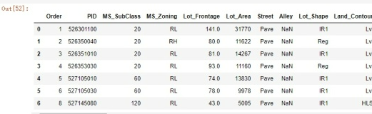
training_data.head(7)

在这里插入图片描述

3 观察各项主要特征与房屋售价的关系

该数据集具有46个类别型变量，34个数值型变量，整理到excel表格中，用于筛选与房价息息相关的变量。从中筛选出以下几个与房价相关的变量：

类别型变量：

Utilities : 可用设施（电、天然气、水）
Heating (Nominal): 暖气类型
Central Air (Nominal): 是否有中央空调
Garage Type (Nominal): 车库位置
Neighborhood (Nominal): Ames市区内的物理位置（地图地段）
Overall Qual (Ordinal): 评估房屋的整体材料和光洁度

数值型变量：

Lot Area（Continuous）：地皮面积（平方英尺）
Gr Liv Area (Continuous): 地面以上居住面积平方英尺
Total Bsmt SF (Continuous): 地下面积的总面积
TotRmsAbvGrd (Discrete): 地面上全部房间数目

分析最重要的变量"SalePrice"

training_data['SalePrice'].describe()

在这里插入图片描述

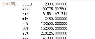
从上面的描述性统计可以看出房价的平均值、标准差、最小值、25%分位数、50%分位数、75%分位数、最大值等，并且SalePrice没有无效或者其他非数值的数据。

#绘制"SalePrice"的直方图
sns.distplot(training_data['SalePrice'])
#计算峰度和偏度
print("Skewness: %f" % training_data['SalePrice'].skew())
print("Kurtosis: %f" % training_data['SalePrice'].kurt())

在这里插入图片描述

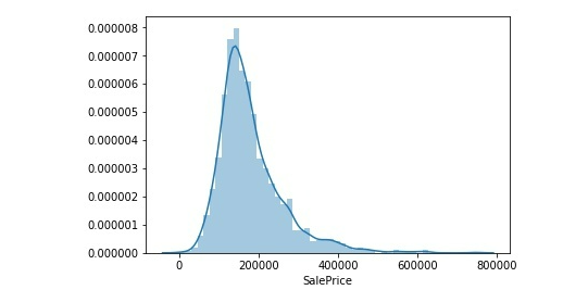
从直方图中可以看出"SalePrice"成正态分布，峰度为4.838055，偏度为1.721408，比正态分布的高峰更加陡峭，偏度为右偏，长尾拖在右边。

2.类别型变量

（1）Utilities与SalePrice

Utilities (Ordinal): Type of utilities available

AllPub All public Utilities (E,G,W,& S)

NoSewr Electricity, Gas, and Water (Septic Tank)

NoSeWa Electricity and Gas Only

ELO Electricity only

#类别型变量
#1.Utilities 
var = 'Utilities'
data = pd.concat([training_data['SalePrice'], training_data[var]], axis=1)
fig = sns.boxplot(x=var, y="SalePrice", data=data)
fig.axis(ymin=0, ymax=800000)

在这里插入图片描述

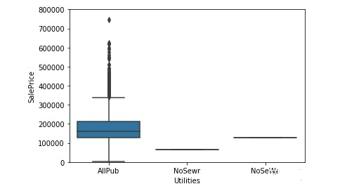
从图中可以看出，配备全套设施（水、电、天然气）的房子价格普遍偏高

（2）Heating与SalePrice

Heating (Nominal): Type of heating

Floor Floor Furnace

GasA Gas forced warm air furnace

GasW Gas hot water or steam heat

Grav Gravity furnace

OthW Hot water or steam heat other than gas

Wall Wall furnace

#2.Heating
var = 'Heating'
data = pd.concat([training_data['SalePrice'], training_data[var]], axis=1)
fig = sns.boxplot(x=var, y="SalePrice", data=data)
fig.axis(ymin=0, ymax=800000)

在这里插入图片描述

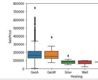
从图中可以看出拥有GasA、GasW的房子价格较高，并且有GasA的房子价格变动较大，房屋价格较高的房子一般都有GasA制暖装置。

（3）Central_Air与SalePrice

#3.Central_Air
var = 'Central_Air'
data = pd.concat([training_data['SalePrice'], training_data[var]], axis=1)
fig = sns.boxplot(x=var, y="SalePrice", data=data)
fig.axis(ymin=0, ymax=800000)

在这里插入图片描述

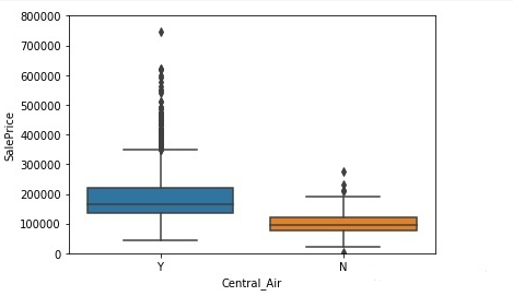
由中央空调的房子能给用户更好的体验，因此一般价格较高，房屋价格较高的房子一般都有中央空调。

（4）Gabage_type与SalePrice

Garage Type (Nominal): Garage location

2Types More than one type of garage

Attchd Attached to home

Basment Basement Garage

BuiltIn Built-In (Garage part of house - typically has room above garage)

CarPort Car Port

Detchd Detached from home

NA No Garage

#4.Gabage_type
var = 'Garage_Type'
data = pd.concat([training_data['SalePrice'], training_data[var]], axis=1)
fig = sns.boxplot(x=var, y="SalePrice", data=data)
fig.axis(ymin=0, ymax=800000)

在这里插入图片描述

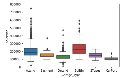
车库越便捷，一般房屋价格越高，临近房屋以及房屋内置的车库这两种价格较高。

（5）Neighborhood与SalePrice

Neighborhood为房屋位于Ames市内的具体的地段，越临近繁华市区、旅游风景区、科技园区、学园区的房屋，房屋价格越贵

#5.Neighborhood
fig, axs = plt.subplots(nrows=2)

sns.boxplot(
    x='Neighborhood',
    y='SalePrice',
    data=training_data.sort_values('Neighborhood'),
    ax=axs[0]
)

sns.countplot(
    x='Neighborhood',
    data=training_data.sort_values('Neighborhood'),
    ax=axs[1]
)

# Draw median price
axs[0].axhline(
    y=training_data['SalePrice'].median(), 
    color='red',
    linestyle='dotted'
)

# Label the bars with counts
for patch in axs[1].patches:
    x = patch.get_bbox().get_points()[:, 0]
    y = patch.get_bbox().get_points()[1, 1]
    axs[1].annotate(f'{int(y)}', (x.mean(), y), ha='center', va='bottom')
    
# Format x-axes
axs[1].set_xticklabels(axs[1].xaxis.get_majorticklabels(), rotation=90)
axs[0].xaxis.set_visible(False)

# Narrow the gap between the plots
plt.subplots_adjust(hspace=0.01)

在这里插入图片描述

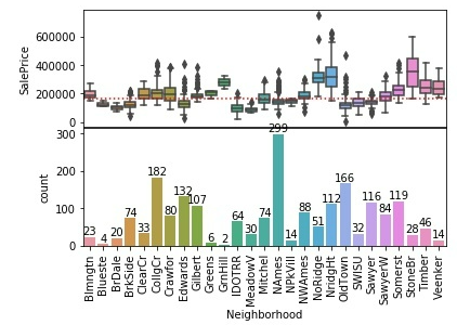
从上图结果可以看出，我们训练数据集中Neighborhood这一列数据不均匀，NAmes有299条数据，而Blueste只有4条数据，Gilbert只有6条数据，GmHill只有2条数据，这样造成数据没那么准确。

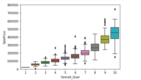
（6）Overall Qual 与SalePrice

总体评价越高，应该房屋的价格越高

#Overall Qual 
var = 'Overall_Qual'
data = pd.concat([training_data['SalePrice'], training_data[var]], axis=1)
fig = sns.boxplot(x=var, y="SalePrice", data=data)
fig.axis(ymin=0, ymax=800000)

在这里插入图片描述

3.数值型变量

（1） Lot Area与SalePrice

#数值型变量
#1.Lot Area
sns.jointplot(
    x='Lot_Area', 
    y='SalePrice', 
    data=training_data,
    stat_func=None,
    kind="reg",
    ratio=4,
    space=0,
    scatter_kws={
        's': 3,
        'alpha': 0.25
    },
    line_kws={
        'color': 'black'
    }
)

在这里插入图片描述

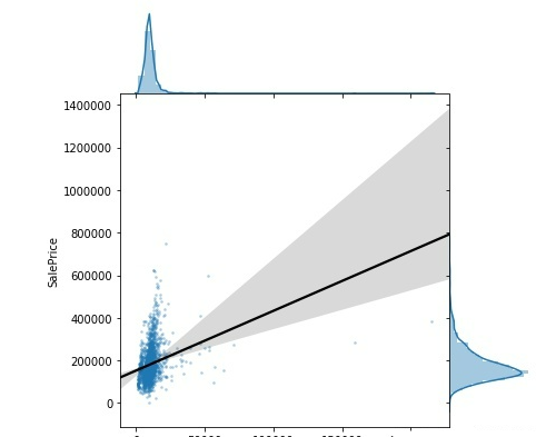
看起来没有什么明显的趋势，散点图主要集中在前半部分，不够分散

（2）Gr_Liv_Area与SalePrice

Gr_Liv_Area代表建筑在土地上的房屋的面积

猜测两者应该成正相关，即房屋面积越大，房屋的价格越高

sns.jointplot(
    x='Gr_Liv_Area', 
    y='SalePrice', 
    data=training_data,
    stat_func=None,
    kind="reg",
    ratio=4,
    space=0,
    scatter_kws={
        's': 3,
        'alpha': 0.25
    },
    line_kws={
        'color': 'black'
    }
)

在这里插入图片描述

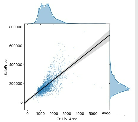
结果：两者的确呈现正相关的线性关系，发现Gr_ Liv_ Area中有处于5000以上的异常值

编写函数，将5000以上的Gr_ Liv_ Area异常值移除

def remove_outliers(data, variable, lower=-np.inf, upper=np.inf):
    """
    Input:
      data (data frame): the table to be filtered
      variable (string): the column with numerical outliers
      lower (numeric): observations with values lower than this will be removed
      upper (numeric): observations with values higher than this will be removed
    
    Output:
      a winsorized data frame with outliers removed
    """
    data=data[(data[variable]>lower)&(data[variable]

再次绘图

在这里插入图片描述

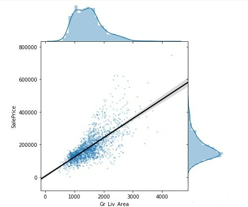
两者的确呈现正相关的线性关系

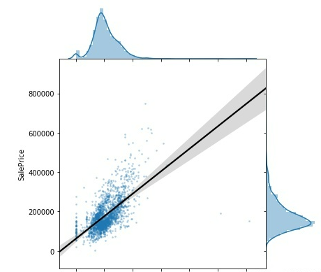
（3）Total_Bsmt_SF与SalePrice

#3.Total Bsmt SF
sns.jointplot(
    x='Total_Bsmt_SF', 
    y='SalePrice', 
    data=training_data,
    stat_func=None,
    kind="reg",
    ratio=4,
    space=0,
    scatter_kws={
        's': 3,
        'alpha': 0.25
    },
    line_kws={
        'color': 'black'
    }
)

在这里插入图片描述

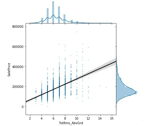
(4)TotRms_AbvGrd与SalePrice

#4.TotRmsAbvGrd
sns.jointplot(
    x='TotRms_AbvGrd', 
    y='SalePrice', 
    data=training_data,
    stat_func=None,
    kind="reg",
    ratio=4,
    space=0,
    scatter_kws={
        's': 3,
        'alpha': 0.25
    },
    line_kws={
        'color': 'black'
    }
)

在这里插入图片描述

4. 绘制相关性矩阵

#绘制相关性矩阵
corrmat = training_data.corr()
f, ax = plt.subplots(figsize=(40, 20))
sns.heatmap(corrmat, vmax=0.8,square=True,cmap="PiYG",center=0.0)

在这里插入图片描述

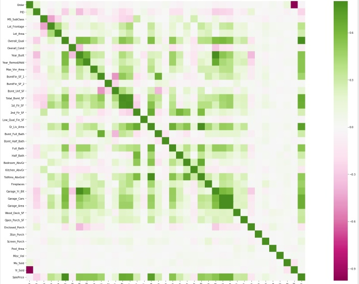
其中数值型变量中，Overall_Qual（房屋的整体评价）、Year_Built（房屋建造年份）、Year_Remod/Add（房屋整修年份）、Mas
Vnr Area（房屋表层砌体模型）、Total_ Bsmt_ SF（地下总面积）、1stFlr_SF（一楼总面积）、 Gr_ L
iv_Area（地上居住面积）、Garage_Cars （车库数量）、Garage_Area（车库面积）都与呈正相关

最后从Year_Built（房屋建造年份）、Year_Remod/Add（房屋整修年份）中选取Year_Built，从1stFlr_SF（一楼总面积）
、 Gr_ L iv_Area（地上居住面积）中选取Gr_ L iv_Area，从Garage_Cars
（车库数量）、Garage_Area（车库面积）中选取Garage_Cars （车库数量）。

6. 拟合模型

sklearn中的回归有多种方法，广义线性回归集中在linear_model库下，例如普通线性回归、Lasso、岭回归等；另外还有其他非线性回归方法，例如核svm、集成方法、贝叶斯回归、K近邻回归、决策树回归、随机森林回归方法等，通过测试各个算法的

（1）加载相应包

#拟合数据
from sklearn import preprocessing
from sklearn import linear_model, svm, gaussian_process
from sklearn.ensemble import RandomForestRegressor
from sklearn.cross_validation import train_test_split
import numpy as np

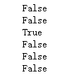
（2）查看各列缺失值

  #查看各列缺失值
    print(training_data.Overall_Qual.isnull().any())
    print(training_data.Gr_Liv_Area.isnull().any())
    print(training_data.Garage_Cars.isnull().any())
    print(training_data.Total_Bsmt_SF.isnull().any())
    print(training_data.Year_Built.isnull().any())
    print(training_data.Mas_Vnr_Area.isnull().any())

发现Total_Bsmt_SF和Mas_Vnr_Area两列有缺失值

   #用均值填补缺失值
    training_data.Total_Bsmt_SF=training_data.Total_Bsmt_SF.fillna(training_data.Total_Bsmt_SF.mean())
    training_data.Mas_Vnr_Area=training_data.Mas_Vnr_Area.fillna(training_data.Mas_Vnr_Area.mean())
    print(training_data.Total_Bsmt_SF.isnull().any())
    print(training_data.Mas_Vnr_Area.isnull().any())

（3）拟合模型

   # 获取数据
    from sklearn import metrics
    cols = ['Overall_Qual','Gr_Liv_Area', 'Garage_Cars','Total_Bsmt_SF', 'Year_Built','Mas_Vnr_Area']
    x = training_data[cols].values
    y = training_data['SalePrice'].values
    X_train,X_test, y_train, y_test = train_test_split(x, y, test_size=0.33, random_state=42)
    
    clf = RandomForestRegressor(n_estimators=400)
    clf.fit(X_train, y_train)
    y_pred = clf.predict(X_test)
    计算MSE：
    print(metrics.mean_squared_error(y_test,y_pred))

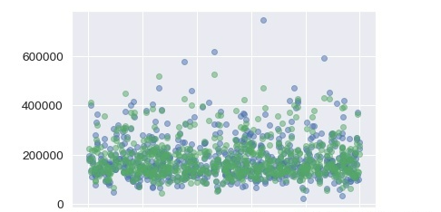
（4）绘制预测结果的散点图

import numpy as np
x = np.random.rand(660)
plt.scatter(x,y_test, alpha=0.5)
plt.scatter(x,y_pred, alpha=0.5,color="G")

在这里插入图片描述

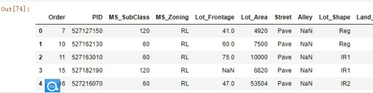
（5）加载测试集数据

test_data=pd.read_csv("ames_test.csv")
test_data.head(5)

在这里插入图片描述

查看缺失值

#查看各列缺失值
print(test_data.Overall_Qual.isnull().any())
print(test_data.Gr_Liv_Area.isnull().any())
print(test_data.Garage_Cars.isnull().any())
print(test_data.Total_Bsmt_SF.isnull().any())
print(test_data.Year_Built.isnull().any())
print(test_data.Mas_Vnr_Area.isnull().any())

#用均值填补缺失值
test_data.Garage_Cars=training_data.Garage_Cars.fillna(training_data.Garage_Cars.mean())
print(test_data.Garage_Cars.isnull().any())

(6)预测测试集的房价

    #预测
    cols = ['Overall_Qual','Gr_Liv_Area', 'Garage_Cars','Total_Bsmt_SF', 'Year_Built','Mas_Vnr_Area']
    x_test_value= test_data[cols].values
    test_pre=clf.predict(x_test_value)
    #写入文件
    prediction = pd.DataFrame(test_pre, columns=['SalePrice'])
    result = pd.concat([test_data['Id'], prediction], axis=1)
    result.to_csv('./Predictions.csv', index=False)

  test_data.Garage_Cars=training_data.Garage_Cars.fillna(training_data.Garage_Cars.mean())
    print(test_data.Garage_Cars.isnull().any())

(6)预测测试集的房价

#预测
cols = ['Overall_Qual','Gr_Liv_Area', 'Garage_Cars','Total_Bsmt_SF', 'Year_Built','Mas_Vnr_Area']
x_test_value= test_data[cols].values
test_pre=clf.predict(x_test_value)
#写入文件
prediction = pd.DataFrame(test_pre, columns=['SalePrice'])
result = pd.concat([test_data['Id'], prediction], axis=1)
result.to_csv('./Predictions.csv', index=False)