🔗 运行环境:Matlab
🚩 撰写作者:左手の明天
🥇 精选专栏:《python》
🔥 推荐专栏:《算法研究》
#### 防伪水印——左手の明天 ####
💗 大家好🤗🤗🤗,我是左手の明天!好久不见💗
💗今天开启新的系列——重新定义matlab强大系列💗
📆 最近更新:2023 年 09 月 24 日,左手の明天的第 292 篇原创博客
📚 更新于专栏:matlab
#### 防伪水印——左手の明天 ####
问题设立
假设有如下数据:
Data = ...
  [0.0000    5.8955
   0.1000    3.5639
   0.2000    2.5173
   0.3000    1.9790
   0.4000    1.8990
   0.5000    1.3938
   0.6000    1.1359
   0.7000    1.0096
   0.8000    1.0343
   0.9000    0.8435
   1.0000    0.6856
   1.1000    0.6100
   1.2000    0.5392
   1.3000    0.3946
   1.4000    0.3903
   1.5000    0.5474
   1.6000    0.3459
   1.7000    0.1370
   1.8000    0.2211
   1.9000    0.1704
   2.0000    0.2636];
利用matlab绘制这些数据点:
t = Data(:,1);
y = Data(:,2);
% axis([0 2 -0.5 6])
% hold on
plot(t,y,'ro')
title('Data points')
% hold off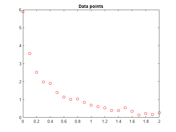
我们要对数据进行
y = c(1)*exp(-lam(1)*t) + c(2)*exp(-lam(2)*t)函数拟合。
使用 lsqcurvefit 的求解方法
lsqcurvefit 函数可以轻松求解这类问题。
首先,定义涉及一个变量 x 的参数:
x(1) = c(1)

x(2) = lam(1)

x(3) = c(2)

x(4) = lam(2)
然后将曲线定义为参数 x 和数据 t 的函数:
F = @(x,xdata)x(1)*exp(-x(2)*xdata) + x(3)*exp(-x(4)*xdata);任意设置一个初始点 x0 如下:c(1) = 1,lam(1) = 1,c(2) = 1,lam(2) = 0:
x0 = [1 1 1 0];运行求解器并绘制拟合结果。
[x,resnorm,~,exitflag,output] = lsqcurvefit(F,x0,t,y)

Local minimum possible.

lsqcurvefit stopped because the final change in the sum of squares relative to
its initial value is less than the value of the function tolerance.

x = 1×4

    3.0068   10.5869    2.8891    1.4003

resnorm = 0.1477
exitflag = 3
output = struct with fields:
      firstorderopt: 7.8852e-06
         iterations: 6
          funcCount: 35
       cgiterations: 0
          algorithm: 'trust-region-reflective'
           stepsize: 0.0096
            message: 'Local minimum possible....'
       bestfeasible: []
    constrviolation: []
hold on
plot(t,F(x,t))
hold off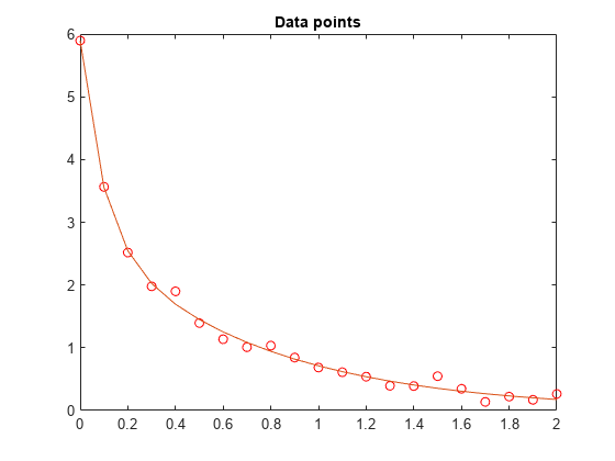
使用 fminunc 的求解方法
为了使用 fminunc 求解问题,将目标函数设置为残差的平方和。
Fsumsquares = @(x)sum((F(x,t) - y).^2);
opts = optimoptions('fminunc','Algorithm','quasi-newton');
[xunc,ressquared,eflag,outputu] = ...
    fminunc(Fsumsquares,x0,opts)
Local minimum found.

Optimization completed because the size of the gradient is less than
the value of the optimality tolerance.
xunc = 1×4

    2.8890    1.4003    3.0069   10.5862

ressquared = 0.1477
eflag = 1
outputu = struct with fields:
       iterations: 30
        funcCount: 185
         stepsize: 0.0017
     lssteplength: 1
    firstorderopt: 2.9662e-05
        algorithm: 'quasi-newton'
          message: 'Local minimum found....'
请注意,fminunc 找到了与 lsqcurvefit 相同的解,但为此进行了更多的函数计算。fminunc 的参数与 lsqcurvefit 的参数顺序相反;较大的 lam 是 lam(2),而不是 lam(1)。这并不奇怪,变量的顺序是任意的。
fprintf(['There were %d iterations using fminunc,' ...
    ' and %d using lsqcurvefit.\n'], ...
    outputu.iterations,output.iterations)


There were 30 iterations using fminunc, and 6 using lsqcurvefit.
fprintf(['There were %d function evaluations using fminunc,' ...
' and %d using lsqcurvefit.'], ...
outputu.funcCount,output.funcCount)
There were 185 function evaluations using fminunc, and 35 using lsqcurvefit.拆分线性和非线性问题
请注意,拟合问题对于参数 c(1) 和 c(2) 是线性的。这意味着对于 lam(1) 和 lam(2) 的任何值,可以使用反斜杠运算符来找到求解最小二乘问题的 c(1) 和 c(2) 的值。
现在将此问题作为二维问题重新处理,搜索 lam(1) 和 lam(2) 的最佳值。在每步中按上面所述使用反斜杠运算符来计算 c(1) 和 c(2) 的值。
type fitvector
function yEst = fitvector(lam,xdata,ydata)
%FITVECTOR  Used by DATDEMO to return value of fitting function.
%   yEst = FITVECTOR(lam,xdata) returns the value of the fitting function, y
%   (defined below), at the data points xdata with parameters set to lam.
%   yEst is returned as a N-by-1 column vector, where N is the number of
%   data points.
%
%   FITVECTOR assumes the fitting function, y, takes the form
%
%     y =  c(1)*exp(-lam(1)*t) + ... + c(n)*exp(-lam(n)*t)
%
%   with n linear parameters c, and n nonlinear parameters lam.
%
%   To solve for the linear parameters c, we build a matrix A
%   where the j-th column of A is exp(-lam(j)*xdata) (xdata is a vector).
%   Then we solve A*c = ydata for the linear least-squares solution c,
%   where ydata is the observed values of y.

A = zeros(length(xdata),length(lam));  % build A matrix
for j = 1:length(lam)
   A(:,j) = exp(-lam(j)*xdata);
end
c = A\ydata; % solve A*c = y for linear parameters c
yEst = A*c; % return the estimated response based on c
使用 lsqcurvefit 求解问题,从二维初始点 lam(1), lam(2) 开始:
x02 = [1 0];
F2 = @(x,t) fitvector(x,t,y);

[x2,resnorm2,~,exitflag2,output2] = lsqcurvefit(F2,x02,t,y)
Local minimum possible.

lsqcurvefit stopped because the final change in the sum of squares relative to
its initial value is less than the value of the function tolerance.
x2 = 1×2

   10.5861    1.4003

resnorm2 = 0.1477
exitflag2 = 3
output2 = struct with fields:
      firstorderopt: 4.4018e-06
         iterations: 10
          funcCount: 33
       cgiterations: 0
          algorithm: 'trust-region-reflective'
           stepsize: 0.0080
            message: 'Local minimum possible....'
       bestfeasible: []
    constrviolation: []
二维求解的效率类似于四维求解的效率:
fprintf(['There were %d function evaluations using the 2-d ' ...
    'formulation, and %d using the 4-d formulation.'], ...
    output2.funcCount,output.funcCount)


There were 33 function evaluations using the 2-d formulation, and 35 using the 4-d formulation.
对于初始估计值来说,拆分问题更稳健
为最初的四参数问题选择的起点不理想会得到局部解,而非全局解。为拆分的两参数问题选择具有同样不理想的 lam(1) 和 lam(2) 值的起点会得到全局解。为了说明这一点,使用会得到相对较差的局部解的起点重新运行原始问题,并将得到的拟合与全局解进行比较。
线性拟合
多项式拟合
多项式拟合就是利用下面形式的方程去拟合数据:

matlab中可以用polyfit()函数进行多项式拟合。
polyfit-多项式曲线拟合
p = polyfit(x,y,n) 返回次数为 n 的多项式 p(x) 的系数,该阶数是 y 中数据的最佳拟合(基于最小二乘指标)。p 中的系数按降幂排列,p 的长度为 n+1
![]()
将多项式与三角函数拟合
在区间 [0,4*pi] 中沿正弦曲线生成 10 个等间距的点。
x = linspace(0,4*pi,10);
y = sin(x);
使用 polyfit 将一个 7 次多项式与这些点拟合。
p = polyfit(x,y,7);在更精细的网格上计算多项式并绘制结果图。
x1 = linspace(0,4*pi);
y1 = polyval(p,x1);
figure
plot(x,y,'o')
hold on
plot(x1,y1)
hold off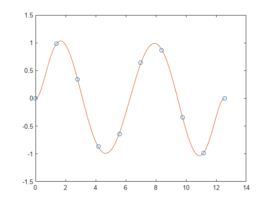
将多项式与点集拟合
创建一个由区间 [0,1] 中的 5 个等间距点组成的向量,并计算这些点处的 y(x)=(1+x)−1。
x = linspace(0,1,5);
y = 1./(1+x);
将 4 次多项式与 5 个点拟合。通常,对于 n 个点,可以拟合 n-1 次多项式以便完全通过这些点。
p = polyfit(x,y,4);在由 0 和 2 之间的点组成的更精细网格上计算原始函数和多项式拟合。
x1 = linspace(0,2);
y1 = 1./(1+x1);
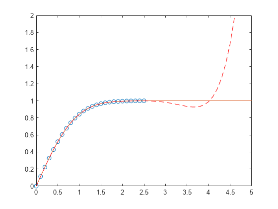
f1 = polyval(p,x1);在更大的区间 [0,2] 中绘制函数值和多项式拟合,其中包含用于获取以圆形突出显示的多项式拟合的点。多项式拟合在原始 [0,1] 区间中的效果较好,但在该区间外部很快与拟合函数出现差异。
figure
plot(x,y,'o')
hold on
plot(x1,y1)
plot(x1,f1,'r--')
legend('y','y1','f1')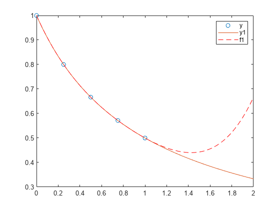
对误差函数进行多项式拟合
首先生成 x 点的向量,在区间 [0,2.5] 内等间距分布;然后计算这些点处的 erf(x)。
x = (0:0.1:2.5)';
y = erf(x);
确定 6 次逼近多项式的系数。
p = polyfit(x,y,6)


p = 1×7

    0.0084   -0.0983    0.4217   -0.7435    0.1471    1.1064    0.0004
为了查看拟合情况如何,在各数据点处计算多项式,并生成说明数据、拟合和误差的一个表。
f = polyval(p,x);
T = table(x,y,f,y-f,'VariableNames',{'X','Y','Fit','FitError'})

T=26×4 table
     X        Y          Fit         FitError
    ___    _______    __________    ___________

      0          0    0.00044117    -0.00044117
    0.1    0.11246       0.11185     0.00060836
    0.2     0.2227       0.22231     0.00039189
    0.3    0.32863       0.32872    -9.7429e-05
    0.4    0.42839        0.4288    -0.00040661
    0.5     0.5205       0.52093    -0.00042568
    0.6    0.60386       0.60408    -0.00022824
    0.7     0.6778       0.67775     4.6383e-05
    0.8     0.7421       0.74183     0.00026992
    0.9    0.79691       0.79654     0.00036515
      1     0.8427       0.84238      0.0003164
    1.1    0.88021       0.88005     0.00015948
    1.2    0.91031       0.91035    -3.9919e-05
    1.3    0.93401       0.93422      -0.000211
    1.4    0.95229       0.95258    -0.00029933
    1.5    0.96611       0.96639    -0.00028097
      ⋮
在该区间中,插值与实际值非常符合。创建
x1 = (0:0.1:5)';
y1 = erf(x1);
f1 = polyval(p,x1);
figure
plot(x,y,'o')
hold on
plot(x1,y1,'-')
plot(x1,f1,'r--')
axis([0  5  0  2])
hold off
一个绘图,以显示在该区间以外,外插值与实际数据值如何快速偏离。
简单线性回归
将一个简单线性回归模型与一组离散二维数据点拟合。
创建几个由样本数据点 (x,y) 组成的向量。对数据进行一次多项式拟合。
x = 1:50;
y = -0.3*x + 2*randn(1,50);
p = polyfit(x,y,1);
计算在 x 中的点处拟合的多项式 p。用这些数据绘制得到的线性回归模型。
f = polyval(p,x);
plot(x,y,'o',x,f,'-')
legend('data','linear fit') 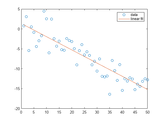
具有误差估计值的线性回归
将一个线性模型拟合到一组数据点并绘制结果,其中包含预测区间为 95% 的估计值。
创建几个由样本数据点 (x,y) 组成的向量。使用 polyfit 对数据进行一次多项式拟合。指定两个输出以返回线性拟合的系数以及误差估计结构体。
x = 1:100;
y = -0.3*x + 2*randn(1,100);
[p,S] = polyfit(x,y,1);
计算以 p 为系数的一次多项式在 x 中各点处的拟合值。将误差估计结构体指定为第三个输入,以便 polyval 计算标准误差的估计值。标准误差估计值在 delta 中返回。
[y_fit,delta] = polyval(p,x,S);绘制原始数据、线性拟合和 95% 预测区间 y±2Δ。
plot(x,y,'bo')
hold on
plot(x,y_fit,'r-')
plot(x,y_fit+2*delta,'m--',x,y_fit-2*delta,'m--')
title('Linear Fit of Data with 95% Prediction Interval')
legend('Data','Linear Fit','95% Prediction Interval')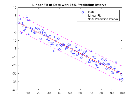
对于多项式拟合,不是阶数越多越好。比如看以下例子,阶数越多,曲线越能够穿过每一个点,但是曲线的形状与理论曲线偏离越大。所以选择最适合的才是最好的。
x=0:0.5:10;
y=0.03*x.^4-0.5*x.^3+2.0*x.^2-0*x-4+6*(rand(size(x))-0.5);
p=polyfit(x,y,4);
x2=0:0.05:10;
y2=polyval(p,x2);
figure();
subplot(1,2,1)
hold on
plot(x,y,'linewidth',1.5,'MarkerSize',15,'Marker','.','color','k')
plot(x,0.03*x.^4-0.5*x.^3+2.0*x.^2-0*x-4,'linewidth',1,'color','b')
hold off
legend('原始数据点','理论曲线','Location','southoutside','Orientation','horizontal')
legend('boxoff')
box on
subplot(1,2,2)
hold on
plot(x2,y2,'-','linewidth',1.5,'color','r')
plot(x,y,'LineStyle','none','MarkerSize',15,'Marker','.','color','k')
hold off
box on
legend('拟合曲线','数据点','Location','southoutside','Orientation','horizontal')
legend('boxoff')
线性拟合
线性拟合就是能够把拟合函数写成下面这种形式的:

其中f(x)是关于x的函数,其表达式是已知的。p是常数系数,这个是未知的。
举个例子

虽然看上去很非线性,但是x和y都是已知的,a、b、c是未知的,而且是线性的,所以可以被非常简单的拟合出来。假设a=2.5,b=0.5,c=-1,加入随机扰动。
x=0:0.5:10;
a=2.5;
b=0.5;
c=-1;

y=a*sin(0.2*x.^2+x)+b*sqrt(x+1)+c+0.5*rand(size(x));


yn1=sin(0.2*x.^2+x);
yn2=sqrt(x+1);
yn3=ones(size(x));
X=[yn1;yn2;yn3];

Pn=X'\y';
yn=Pn(1)*yn1+Pn(2)*yn2+Pn(3)*yn3;

figure()
subplot(1,2,1)
plot(x,y,'linewidth',1.5,'MarkerSize',15,'Marker','.','color','k')
legend('原始数据点','Location','southoutside','Orientation','horizontal')
legend('boxoff')
subplot(1,2,2)
hold on
x2=0:0.01:10;
plot(x2,Pn(1)*sin(0.2*x2.^2+x2)+Pn(2)*sqrt(x2+1)+Pn(3),'-','linewidth',1.5,'color','r')
plot(x,y,'LineStyle','none','MarkerSize',15,'Marker','.','color','k')
hold off
box on
legend('拟合曲线','数据点','Location','southoutside','Orientation','horizontal')
legend('boxoff')
拟合的最终效果为:

最终得到的拟合参数为:a=2.47,b=0.47,c=-0.66。