学过高斯软件的人都知道,我们在撰写输入文件 gjf 时需要准备输入【泛函】和【基组】这两个关键词。
【泛函】敲定计算方法,【基组】则类似格点积分中的密度,与计算精度密切相关。
部分研究人员借用高斯中的一系列基组去包装输入几何信息(距离、角度和二面角),这样做一方面提高了GNN的可解释性,另一方面也实实在在的提高了模型精度。从 AI 角度看,embedding则可以看作是几何信息的升维。
具体来说:
- 如果模型输入仅有距离信息,则采用径向基函数去embedding。常用的有 Gaussian ,也有Bessel
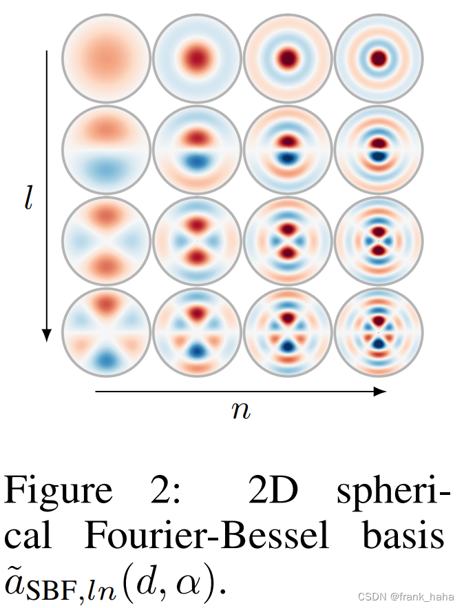
- 如果模型输入含有距离和角度信息。在直角坐标系下,可以用 Gaussian 和 sin 函数组embedding。在球坐标系下,可以考虑 spherical Bessel functions and spherical harmonics 组合。其中 spherical harmonics 采用m=0的形式。
- 如果模型输入含有距离,角度和二面角信息,一般采用 spherical Bessel functions and spherical harmonics 组合。可能有其他的,但目前涉及二面角的模型较少,据我了解,Spherenet和ComENet均采用的是这种组合。
下面进行简要介绍:
Gaussian 系列基组
SchNet网络架构中使用的基组,是目前用途最广的基组之一。
我们借助 DIG 框架中 schnet 的实现,对其进行可视化:
from dig.threedgraph.method.schnet.schnet import *

import numpy as np
import math
import matplotlib.pyplot as plt

import torch


dist_test = torch.arange(0.01, 5.01, 0.01)
dist_emb = emb(num_gaussians=5)
y = dist_emb(dist_test)
y = y.T

for idx, y_plot in enumerate(y):
    x = [a_dist.detach().numpy() for a_dist in dist_test]
    y = [an_emb.detach().numpy() for an_emb in y_plot]

    plt.plot(x, y, label=f"Gaussian embedding {idx}")

plt.xlabel("x")
plt.ylabel("y")
plt.legend()
plt.show()
结果如下图所示:
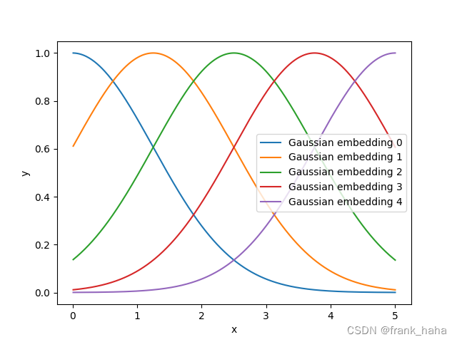
所谓,“对几何信息进行嵌入”,指,同一个距离信息对应x轴一个点。如果高斯基组有5,则,嵌入后,该距离信息就映射到了5个口袋里,获得一组长度为5的特征向量。
此处为了清晰的可视化,仅设置 num_gaussians=5 ,在实际应用中,这一数值往往设的很高。例如,原版的 schnet 将这一数值设为 300,在 DIG 版本中,这一数值是默认的 50,而在最新的 schnetpack 中,这一数值 降为了 20.
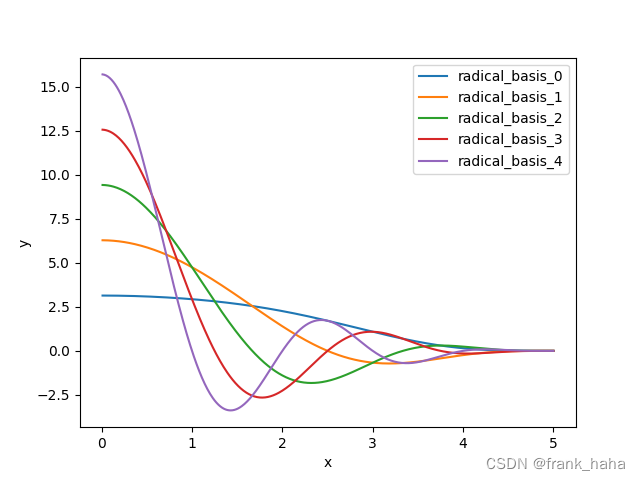
Bessel 系列基组
与高斯基组类似,Bessel 系列基组用于 embedding 距离信息,文献里用 spherical Bessel functions 表示。
其源头可以追溯到微分方程的求解,spherical Bessel functions 是作为一系列解中的径向部分存在,也常被称为 radical Bessel functions。
最早使用 Bessel functions 的(可能不严谨)GNN大概是 DimeNet。据 DimeNet 原文报道,使用 Bessel functions 会带来一定程度的精度提升。
我们借助 DIG 框架中 DimeNet 的实现,对其进行可视化:
from dig.threedgraph.method.spherenet.features import *

import numpy as np
import math
import matplotlib.pyplot as plt

import torch

dist_test = torch.arange(0.01, 5.01, 0.01)
dist_emb = dist_emb(num_radial=5)
y = dist_emb(dist_test)
y = y.T

for idx, y_plot in enumerate(y):
    x = [a_dist.detach().numpy() for a_dist in dist_test]
    y = [an_emb.detach().numpy() for an_emb in y_plot]

    plt.plot(x, y, label=f"radical_basis_{idx}")

plt.xlabel("x")
plt.ylabel("y")
plt.legend()
plt.show()
结果如下图所示:
spherical harmonics 基组
spherical Bessel functions 和 spherical harmonics 不是一个基组。他俩分别对应方程特解中的径向和角度部分。
(下图为 ComENet 中的概述)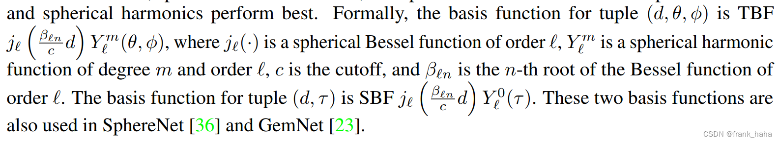
spherical harmonics 基组常常在球极坐标系下,和 spherical Bessel functions 配套使用。
如果输入的几何信息仅有角度,没有二面角,我们将 spherical harmonics 中的 m 置零。
此时得到的是一系列二维的 embedding 矩阵。
我们借助 DIG 框架中 SphereNet 的实现,对其进行可视化(源码稍微改了改,此处仅是一些思路):
from dig.threedgraph.method.spherenet.features import *

import numpy as np
import math
import matplotlib.pyplot as plt

import torch

angle_emb = angle_emb(num_spherical=4, num_radial=4, cutoff=4)
rlist = np.arange(0, 4.01, 0.005)  # Angstroms
thetalist = np.radians(np.arange(0, 361, 0.5))  # Radians
rmesh, thetamesh = np.meshgrid(rlist, thetalist)  # Generate a mesh

n = 1
l = 1
fig = plt.figure()
info = angle_emb(torch.tensor(rlist), torch.tensor(thetalist))
info_0 = info[n, l]
info_0 = info_0.detach().numpy()

info_0 = info_0.reshape(len(rlist), len(thetalist))
info_0 = info_0.T
fig, ax = plt.subplots(subplot_kw=dict(projection='polar'))
ax.contourf(thetamesh, rmesh, info_0, 100, cmap='RdBu')
ax.set_rticks([])
ax.set_xticks([])
plt.savefig(f'./basis/n_{n}_l_{l}.png', dpi=400)
结果如下图所示:
我们可以得到一系列能够embedding角度和距离信息的函数。
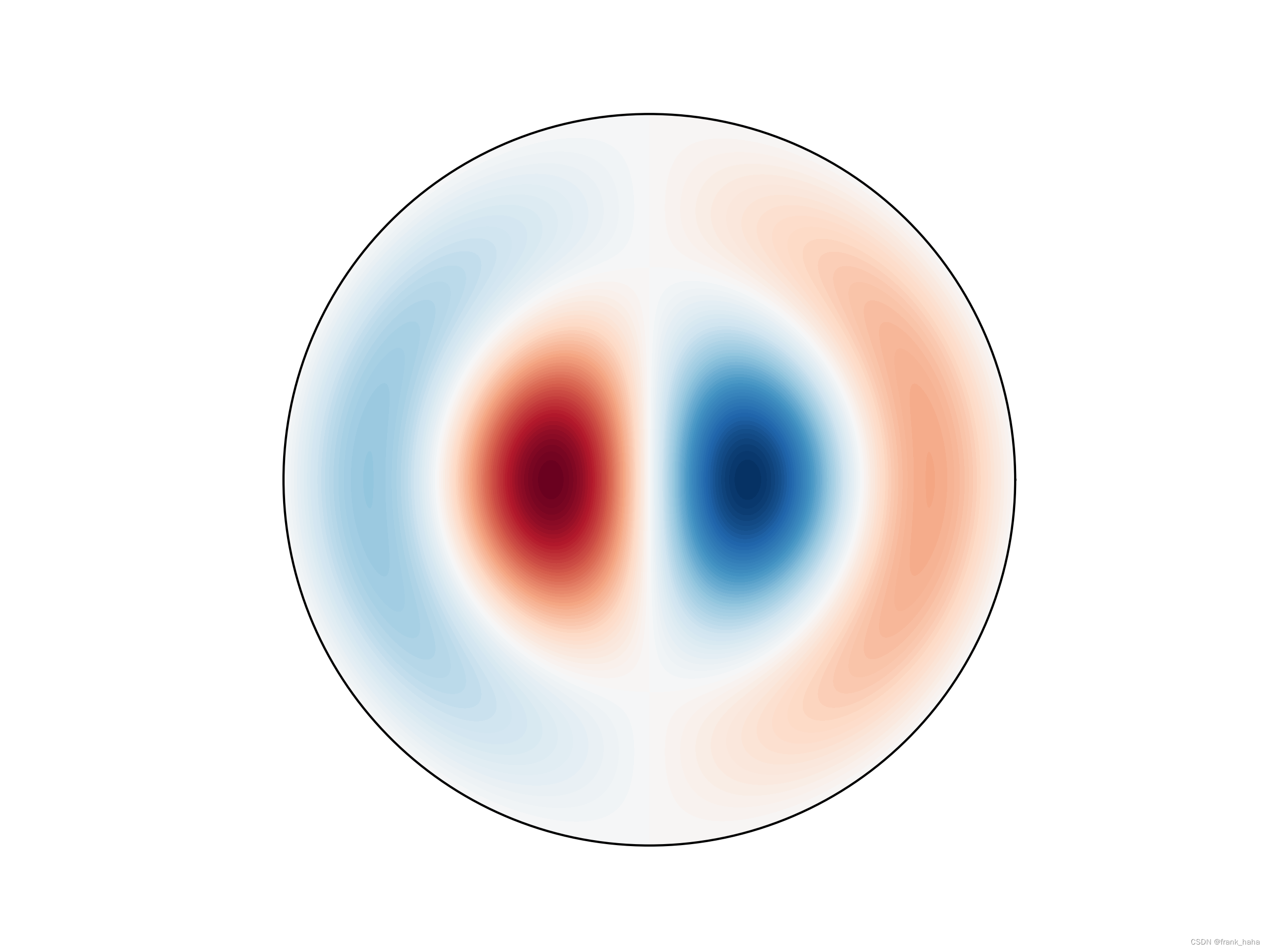
下图是DimeNet原文中的图:
需要注意的是,DimeNet源码中对 l=0 的径向函数进行了修改,所以无法复现 Figure 2 第一行。
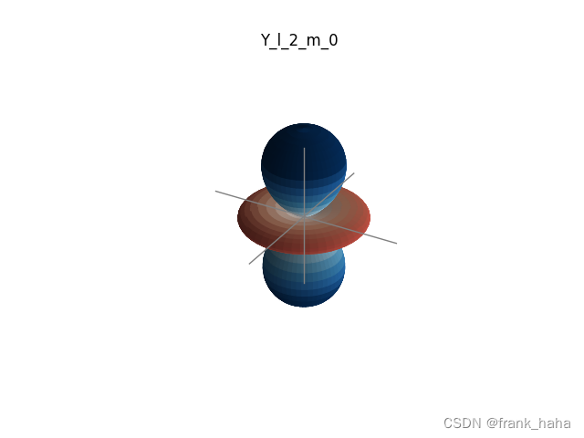
我们还可以借助 scipy 进行实现,例如,下面我们对角度部分 ( spherical harmonics )进行可视化(不涉及径向部分,径向部分在 scipy.special._spherical_bessel 里):
- 借用plotly实现可交互的可视化
import plotly.graph_objects as go
import numpy as np
from mpl_toolkits.mplot3d import Axes3D
from scipy.special import sph_harm

# from scipy.special._spherical_bessel import


# l, m = 3, 0

for l in range(0, 4):
    for m in range(-l, l+1):
        theta = np.linspace(0, np.pi, 100)
        phi = np.linspace(0, 2 * np.pi, 100)
        theta, phi = np.meshgrid(theta, phi)
        xyz = np.array([np.sin(theta) * np.sin(phi),
                        np.sin(theta) * np.cos(phi),
                        np.cos(theta)])

        Y = sph_harm(abs(m), l, phi, theta)

        if m < 0:
            Y = np.sqrt(2) * (-1) ** m * Y.imag
        elif m > 0:
            Y = np.sqrt(2) * (-1) ** m * Y.real
        Yx, Yy, Yz = np.abs(Y) * xyz

        fig = go.Figure(data=[go.Surface(x=Yx, y=Yy, z=Yz, surfacecolor=Y.real), ])

        fig.update_layout(title=f'Y_l_{l}_m_{m}', )

        fig.write_html(rf'./pics_html/Y_l_{l}_m_{m}.html')
- 借用matplotlib实现静态的可视化:
import numpy as np
import matplotlib.pyplot as plt
import matplotlib.gridspec as gridspec
# The following import configures Matplotlib for 3D plotting.
from mpl_toolkits.mplot3d import Axes3D
from scipy.special import sph_harm


# plt.rc('text', usetex=True)

# Grids of polar and azimuthal angles
theta = np.linspace(0, np.pi, 100)
phi = np.linspace(0, 2*np.pi, 100)
# Create a 2-D meshgrid of (theta, phi) angles.
theta, phi = np.meshgrid(theta, phi)
# Calculate the Cartesian coordinates of each point in the mesh.
xyz = np.array([np.sin(theta) * np.sin(phi),
                np.sin(theta) * np.cos(phi),
                np.cos(theta)])

def plot_Y(ax, el, m):
    """Plot the spherical harmonic of degree el and order m on Axes ax."""

    # NB In SciPy's sph_harm function the azimuthal coordinate, theta,
    # comes before the polar coordinate, phi.
    Y = sph_harm(abs(m), el, phi, theta)

    # Linear combination of Y_l,m and Y_l,-m to create the real form.
    if m < 0:
        Y = np.sqrt(2) * (-1)**m * Y.imag
    elif m > 0:
        Y = np.sqrt(2) * (-1)**m * Y.real
    Yx, Yy, Yz = np.abs(Y) * xyz

    # Colour the plotted surface according to the sign of Y.
    cmap = plt.cm.ScalarMappable(cmap='RdBu')
    cmap.set_clim(-0.5, 0.5)

    ax.plot_surface(Yx, Yy, Yz,
                    facecolors=cmap.to_rgba(Y.real),
                    rstride=2, cstride=2)

    # Draw a set of x, y, z axes for reference.
    ax_lim = 0.5
    ax.plot([-ax_lim, ax_lim], [0,0], [0,0], c='0.5', lw=1, zorder=10)
    ax.plot([0,0], [-ax_lim, ax_lim], [0,0], c='0.5', lw=1, zorder=10)
    ax.plot([0,0], [0,0], [-ax_lim, ax_lim], c='0.5', lw=1, zorder=10)
    # Set the Axes limits and title, turn off the Axes frame.
    # ax.set_title(r'$Y_{{{},{}}}$'.format(el, m))
    ax.set_title('Y_l_{}_m_{}'.format(el, m))
    ax_lim = 0.5
    ax.set_xlim(-ax_lim, ax_lim)
    ax.set_ylim(-ax_lim, ax_lim)
    ax.set_zlim(-ax_lim, ax_lim)
    ax.axis('off')

# fig = plt.figure(figsize=plt.figaspect(1.))

for l in range(0, 4):
    for m in range(-l, l+1):
        fig = plt.figure()
        ax = fig.add_subplot(projection='3d')
        plot_Y(ax, l, m)
        plt.savefig('./pics_png/Y_l_{}_m_{}.png'.format(l, m))
静态效果如下:
OK,至此,GNN中常用的基组(至少我所了解到的)介绍完了。
一般来说,仅涉及距离信息的架构常常采用 gaussian 基组。
如果要用 spherical harmonics 这种涉及角度的基组,一般需要将几何坐标转到球极坐标下,而这将导致网络适应等变架构时遇到困难。
当然,还有使用 tensor field 做基组的,这块我还了解的少,但看起来好像也是套的 spherical harmonics 。