Reinforcement Learning with Code
This note records how the author begin to learn RL. Both theoretical understanding and code practice are presented. Many material are referenced such as ZhaoShiyu’s Mathematical Foundation of Reinforcement Learning, .
文章目录
- Reinforcement Learning with Code
- Chapter 7. Temporal-Difference Learning
- 7.1 TD leaning of state value
- 7.2 TD learning of action value: Sarsa
- 7.3 TD learning of action value: Expected Sarsa
- 7.4 TD learning of action values: n n n-step Sarsa
- 7.5 TD learning of optimal action values: Q-learning
- Reference
Chapter 7. Temporal-Difference Learning
Temporal-difference (TD) algorithms can be seen as special Robbins-Monro (RM) algorithm solving expectation form of Bellman or Bellman optimality equation.
7.1 TD leaning of state value
Recall the Bellman equation in section 2.2
v π ( s ) = ∑ a π ( a ∣ s ) ( ∑ r p ( r ∣ s , a ) r + γ ∑ s ′ p ( s ′ ∣ s , a ) v π ( s ′ ) ) (elementwise form) v π = r π + γ P π v π (matrix-vector form) v_\pi(s) = \sum_a \pi(a|s) \Big(\sum_rp(r|s,a)r + \gamma \sum_{s^\prime}p(s^\prime|s,a)v_\pi(s^\prime) \Big) \quad \text{(elementwise form)} \\ v_\pi = r_\pi + \gamma P_\pi v_\pi \quad \text{(matrix-vector form)} vπ(s)=a∑π(a∣s)(r∑p(r∣s,a)r+γs′∑p(s′∣s,a)vπ(s′))(elementwise form)vπ=rπ+γPπvπ(matrix-vector form)
where
[ r π ] s ≜ ∑ a π ( a ∣ s ) ∑ r p ( r ∣ s , a ) r [ P π ] s , s ′ = ∑ a π ( a ∣ s ) ∑ s ′ p ( s ′ ∣ s , a ) [r_\pi]_s \triangleq \sum_a \pi(a|s) \sum_r p(r|s,a)r \qquad [P_\pi]_{s,s^\prime} = \sum_a \pi(a|s) \sum_{s^\prime} p(s^\prime|s,a) [rπ]s≜a∑π(a∣s)r∑p(r∣s,a)r[Pπ]s,s′=a∑π(a∣s)s′∑p(s′∣s,a)
Recall the definition of state value: state value is defined as the mean of all possible returns starting from a state, which is actually the expectation of return from a specific state. We can rewrite the above equation into
v π = E [ R + γ v π ] (matrix-vector form) v π ( s ) = E [ R + γ v π ( S ′ ) ∣ S = s ] , s ∈ S (elementwise form) \textcolor{red}{v_\pi = \mathbb{E}[R+\gamma v_\pi]} \quad \text{(matrix-vector form)} \\ \textcolor{red}{v_\pi(s) = \mathbb{E}[R+\gamma v_\pi(S^\prime)|S=s]}, \quad s\in\mathcal{S} \quad \text{(elementwise form)} vπ=E[R+γvπ](matrix-vector form)vπ(s)=E[R+γvπ(S′)∣S=s],s∈S(elementwise form)
where S , S ′ S,S^\prime S,S′ and R R R are the random variables representing the current state, next state and immediate reward. This equation also called the Bellman expectation equation.
We can use Robbins-Monro algorithm introduced in chapter 6 to solve the Bellman expectation equation. Reformulate the problem that is to find the root v π ( s ) v_\pi(s) vπ(s) of equation g ( v π ( s ) ) = v π ( s ) − E [ R + γ v π ( S ′ ) ∣ S = s ] = 0 g(v_\pi(s))=v_\pi(s) - \mathbb{E}[R+\gamma v_\pi(S^\prime)|S=s]=0 g(vπ(s))=vπ(s)−E[R+γvπ(S′)∣S=s]=0, where S ′ S^\prime S′ is iid with s s s. We can only get the measurement with noise
g ~ ( v π ( s ) , η ) = v π ( s ) − ( r + γ v π ( s ′ ) ) = v π ( s ) − E [ R + γ v π ( S ′ ) ∣ S = s ] ⏟ g ( v π ( s ) ) + ( E [ R + γ v π ( S ′ ) ∣ S = s ] − [ r + γ v π ( s ′ ) ] ) ⏟ η \begin{aligned} \tilde{g}(v_\pi(s),\eta) & = v_\pi(s) - (r+\gamma v_\pi(s^\prime)) \\ & = \underbrace{v_\pi(s) - \mathbb{E}[R+\gamma v_\pi(S^\prime)|S=s]}_{g(v_\pi(s))} + \underbrace{\Big( \mathbb{E}[R+\gamma v_\pi(S^\prime)|S=s] - [r+\gamma v_\pi(s^\prime)] \Big)}_{\eta} \end{aligned} g~(vπ(s),η)=vπ(s)−(r+γvπ(s′))=g(vπ(s)) vπ(s)−E[R+γvπ(S′)∣S=s]+η (E[R+γvπ(S′)∣S=s]−[r+γvπ(s′)])
Hence, according to the Robbins-Monro algorithm, we can get the TD learning algorithm as
v k + 1 ( s ) = v k ( s ) − α k ( v k ( s ) − [ r k + γ v π ( s k ′ ) ] ) v_{k+1}(s) = v_k(s) - \alpha_k \Big(v_k(s) - [r_k+\gamma v_\pi(s^\prime_k)] \Big) vk+1(s)=vk(s)−αk(vk(s)−[rk+γvπ(sk′)])
We do some modification in order to remove some assumptions of TD learning. One modification is the sample data { ( s , r k , s k ′ ) } \{(s,r_k,s_k^\prime) \} {(s,rk,sk′)} is changed to { ( s t , r t + 1 , s t + 1 ) } \{(s_t, r_{t+1}, s_{t+1}) \} {(st,rt+1,st+1)}. Due to the modification the algorithm is called temporal-difference learning. Rewrite it in a more concise way:
TD learning : { v t + 1 ( s t ) ⏟ new estimation = v t ( s t ) ⏟ current estimation − α t ( s t ) [ v t ( s t ) − ( r t + 1 + γ v t ( s t + 1 ) ) ⏟ TD target v ˉ t ] ⏞ TD error or Innovation δ t v t + 1 ( s ) = v t ( s ) , for all s ≠ s t \text{TD learning} : \left \{ \begin{aligned} \textcolor{red}{\underbrace{v_{t+1}(s_t)}_{\text{new estimation}}} & \textcolor{red}{= \underbrace{v_t(s_t)}_{\text{current estimation}} - \alpha_t(s_t) \overbrace{\Big[v_t(s_t) - \underbrace{(r_{t+1} +\gamma v_t(s_{t+1}))}_{\text{TD target } \bar{v}_t} \Big]}^{\text{TD error or Innovation } \delta_t}} \\ \textcolor{red}{v_{t+1}(s)} & \textcolor{red}{= v_t(s)}, \quad \text{for all } s\ne s_t \end{aligned} \right. TD learning:⎩ ⎨ ⎧new estimation vt+1(st)vt+1(s)=current estimation vt(st)−αt(st)[vt(st)−TD target vˉt (rt+1+γvt(st+1))] TD error or Innovation δt=vt(s),for all s=st
where t = 0 , 1 , 2 , … t=0,1,2,\dots t=0,1,2,…. Here, v t ( s t ) v_t(s_t) vt(st) is the estimated state value of v π ( s t ) v_\pi(s_t) vπ(st) and a t ( s t ) a_t(s_t) at(st) is the learning rate of s t s_t st at time t t t. And
v ˉ t ≜ r t + 1 + γ v ( s t + 1 ) \bar{v}_t \triangleq r_{t+1}+\gamma v(s_{t+1}) vˉt≜rt+1+γv(st+1)
is called the TD target and
δ t ≜ v ( s t ) − [ r t + 1 + γ v ( s t + 1 ) ] = v ( s t ) − v ˉ t \delta_t \triangleq v(s_t) - [r_{t+1}+\gamma v(s_{t+1})] = v(s_t) - \bar{v}_t δt≜v(st)−[rt+1+γv(st+1)]=v(st)−vˉt
is called the TD error. TD error reflects the deficiency between the current estimate v t v_t vt and the true state value v π v_\pi vπ.
7.2 TD learning of action value: Sarsa
Sarsa is an algorithm directly estimate action values. Estimating action value is important because the policy can be improved based on action values.
Recall the Bellman equation of action value in section 2.5
q π ( s , a ) = ∑ r p ( r ∣ s , a ) r + γ ∑ s ′ p ( s ′ ∣ s , a ) v π ( s ′ ) (elementwise form) = ∑ r p ( r ∣ s , a ) r + γ ∑ s ′ p ( s ′ ∣ s , a ) ∑ a ′ ∈ A ( s ′ ) π ( a ′ ∣ s ′ ) q π ( s ′ , a ′ ) (elementwise form) \begin{aligned} q_\pi(s,a) & =\sum_r p(r|s,a)r + \gamma\sum_{s^\prime} p(s^\prime|s,a) v_\pi(s^\prime) \quad \text{(elementwise form)} \\ & = \sum_r p(r|s,a)r + \gamma\sum_{s^\prime} p(s^\prime|s,a) \sum_{a^\prime \in \mathcal{A}(s^\prime)}\pi(a^\prime|s^\prime) q_\pi(s^\prime,a^\prime) \quad \text{(elementwise form)} \end{aligned} qπ(s,a)=r∑p(r∣s,a)r+γs′∑p(s′∣s,a)vπ(s′)(elementwise form)=r∑p(r∣s,a)r+γs′∑p(s′∣s,a)a′∈A(s′)∑π(a′∣s′)qπ(s′,a′)(elementwise form)
Due to the conditional probability p ( a , b ) = p ( b ) p ( a ∣ b ) p(a,b)=p(b)p(a|b) p(a,b)=p(b)p(a∣b), we have
p ( s ′ , a ′ ∣ s , a ) = p ( s ′ ∣ s , a ) p ( a ′ ∣ s ′ , s , a ) (conditional probility) = p ( s ′ ∣ s , a ) p ( a ′ ∣ s ′ ) (due to conditional independence) = p ( s ′ ∣ s , a ) π ( a ′ ∣ s ′ ) \begin{aligned} p(s^\prime, a^\prime |s,a) & = p(s^\prime|s,a)p(a^\prime|s^\prime, s, a) \quad \text{(conditional probility)} \\ & = p(s^\prime|s,a) p(a^\prime|s^\prime) \quad \text{(due to conditional independence)} \\ & = p(s^\prime|s,a) \pi(a^\prime|s^\prime) \end{aligned} p(s′,a′∣s,a)=p(s′∣s,a)p(a′∣s′,s,a)(conditional probility)=p(s′∣s,a)p(a′∣s′)(due to conditional independence)=p(s′∣s,a)π(a′∣s′)
Due to the above equation, we have
q π ( s , a ) = ∑ r p ( r ∣ s , a ) r + γ ∑ s ′ ∑ a ′ p ( s ′ , a ′ ∣ s , a ) q π ( s ′ , a ′ ) q_\pi(s,a) = \sum_r p(r|s,a)r + \gamma \sum_{s^\prime} \sum_{a^\prime} p(s^\prime,a^\prime|s,a) q_\pi(s^\prime,a^\prime) qπ(s,a)=r∑p(r∣s,a)r+γs′∑a′∑p(s′,a′∣s,a)qπ(s′,a′)
Regard the probability p ( r ∣ s , a ) p(r|s,a) p(r∣s,a) and p ( s ′ , a ′ ∣ s , a ) p(s^\prime, a^\prime |s,a) p(s′,a′∣s,a) as the distribution of random variable R R R and S ′ S^\prime S′ respectively. Then rewrite above equation into expectation form
q π ( s , a ) = E [ R + γ q π ( S ′ , A ′ ) ∣ S = s , A = a ] , for all s , a (expectation form) \textcolor{red}{ q_\pi(s,a) = \mathbb{E}\Big[ R + \gamma q_\pi(S^\prime,A^\prime) \Big| S=s, A=a\Big] }, \text{ for all }s,a \quad \text{(expectation form)} qπ(s,a)=E[R+γqπ(S′,A′) S=s,A=a], for all s,a(expectation form)
where R , S , S ′ R,S,S^\prime R,S,S′ are random variables, denote immediate reward, currnet state and next state respectively.
Hence, we can use the Robbins-Monro algorithm to sovle the Bellamn eqaution of action value. We can define
g ( q π ( s , a ) ) ≜ q π ( s , a ) − E [ R + γ q π ( S ′ , A ′ ) ∣ S = s , A = a ] g(q_\pi(s,a)) \triangleq q_\pi(s,a) - \mathbb{E}{\Big[ R + \gamma q_\pi(S^\prime,A^\prime) \Big| S=s, A=a\Big]} g(qπ(s,a))≜qπ(s,a)−E[R+γqπ(S′,A′) S=s,A=a]
We only can get the observation with noise that
g ~ ( q π ( s , a ) , η ) = q π ( s , a ) − [ r + γ q π ( s ′ , a ′ ) ] = q π ( s , a ) − E [ R + γ q π ( S ′ , A ′ ) ∣ S = s , A = a ] ⏟ g ( q π ( s , a ) ) + [ E [ R + γ q π ( S ′ , A ′ ) ∣ S = s , A = a ] − [ r + γ q π ( s ′ , a ′ ) ] ] ⏟ η \begin{aligned} \tilde{g}\Big(q_\pi(s,a),\eta \Big) & = q_\pi(s,a) - \Big[r+\gamma q_\pi(s^\prime,a^\prime) \Big] \\ & = \underbrace{q_\pi(s,a) - \mathbb{E}{\Big[ R + \gamma q_\pi(S^\prime,A^\prime)\Big| S=s, A=a\Big]}}_{g(q_\pi(s,a))} + \underbrace{\Bigg[\mathbb{E}{\Big[ R + \gamma q_\pi(S^\prime,A^\prime) \Big| S=s, A=a\Big]} - \Big[r+\gamma q_\pi(s^\prime,a^\prime)\Big] \Bigg]}_{\eta} \end{aligned} g~(qπ(s,a),η)=qπ(s,a)−[r+γqπ(s′,a′)]=g(qπ(s,a)) qπ(s,a)−E[R+γqπ(S′,A′) S=s,A=a]+η [E[R+γqπ(S′,A′) S=s,A=a]−[r+γqπ(s′,a′)]]
Hence, according to the Robbins-Monro algorithm, we can get Sarsa as
q k + 1 ( s , a ) = q k ( s , a ) − α k [ q k ( s , a ) − ( r k + γ q k ( s k ′ , a k ′ ) ) ] q_{k+1}(s,a) = q_k(s,a) - \alpha_k \Big[ q_k(s,a) - \big(r_k+\gamma q_k(s^\prime_k,a^\prime_k) \big) \Big] qk+1(s,a)=qk(s,a)−αk[qk(s,a)−(rk+γqk(sk′,ak′))]
Similar to the TD learning estimates state value in last section, we do some modification in above equation. The sampled data ( s , a , r k , s k ′ , a k ′ ) (s,a,r_k,s^\prime_k,a^\prime_k) (s,a,rk,sk′,ak′) is changed to ( s t , a t , r t + 1 , s t + 1 , a t + 1 ) (s_t,a_t,r_{t+1},s_{t+1},a_{t+1}) (st,at,rt+1,st+1,at+1). Hence, the Sarsa becomes
Sarsa : { q t + 1 ( s t , a t ) = q t ( s t , a t ) − α t ( s t , a t ) [ q t ( s t , a t ) − ( r t + 1 + γ q t ( s t + 1 , a t + 1 ) ) ] q t + 1 ( s , a ) = q t ( s , a ) , for all ( s , a ) ≠ ( s t , a t ) \text{Sarsa} : \left \{ \begin{aligned} \textcolor{red}{q_{t+1}(s_t,a_t)} & \textcolor{red}{= q_t(s_t,a_t) - \alpha_t(s_t,a_t) \Big[q_t(s_t,a_t) - (r_{t+1} +\gamma q_t(s_{t+1},a_{t+1})) \Big]} \\ \textcolor{red}{q_{t+1}(s,a)} & \textcolor{red}{= q_t(s,a)}, \quad \text{for all } (s,a) \ne (s_t,a_t) \end{aligned} \right. Sarsa:⎩ ⎨ ⎧qt+1(st,at)qt+1(s,a)=qt(st,at)−αt(st,at)[qt(st,at)−(rt+1+γqt(st+1,at+1))]=qt(s,a),for all (s,a)=(st,at)
where t = 0 , 1 , 2 , … t=0,1,2,\dots t=0,1,2,…. Here, q t ( s , a t ) q_t(s,a_t) qt(s,at) is the estimated action value of ( s t , a t ) (s_t,a_t) (st,at); α t ( s t , a t ) \alpha_t(s_t,a_t) αt(st,at) is the learning rate depending on s t , a t s_t,a_t st,at.
Sarsa is nothing but an action-value version of the TD algorithm. Sarsa is also implemented with policy improvement steps such as ϵ \epsilon ϵ- greedy algorithm. There is a point that should be noticed. In the q q q-value update step, unlike the model-based policy iteration or value iteration algorithm where the values of all states are updated in each iteration, Sarsa only updates a single state-action pair that is visited at time step t t t.
Pesudocode:

7.3 TD learning of action value: Expected Sarsa
Recall the Bellman equation of action value
q π ( s , a ) = ∑ r p ( r ∣ s , a ) r + γ ∑ s ′ p ( s ′ ∣ s , a ) v π ( s ′ ) (elementwise form) q_\pi(s,a) = \sum_r p(r|s,a)r + \gamma\sum_{s^\prime} p(s^\prime|s,a) v_\pi(s^\prime) \quad \text{(elementwise form)} qπ(s,a)=r∑p(r∣s,a)r+γs′∑p(s′∣s,a)vπ(s′)(elementwise form)
Regard the probability p ( r ∣ s , a ) p(r|s,a) p(r∣s,a) and p ( s ′ ∣ s , a ) p(s^\prime|s,a) p(s′∣s,a) as the distribution of random variable R R R and v π ( S ′ ) v_\pi(S^\prime) vπ(S′). Then, we have the expectation form of Bellman equation of action value.
q π ( s , a ) = E [ R + γ v π ( S ′ ) ∣ S = s , A = a ] (expectation form) ( 1 ) q_\pi(s,a) = \mathbb{E}[R + \gamma v_\pi(S^\prime)|S=s,A=a] \quad \text{(expectation form)} \quad (1) qπ(s,a)=E[R+γvπ(S′)∣S=s,A=a](expectation form)(1)
According to the definition of state value we have
E [ q π ( s , A ) ∣ s ] = ∑ a ∈ A ( s ) π ( a ∣ s ) q π ( s , a ) = v π ( s ) → E [ q π ( S ′ , A ) ∣ S ′ ] = v π ( S ′ ) ( 2 ) \begin{aligned} \mathbb{E}[q_\pi(s, A) | s] & = \sum_{a\in\mathcal{A}(s)} \pi(a|s) q_\pi(s,a) = v_\pi(s) \\ \to \mathbb{E}[q_\pi(S^\prime, A) | S^\prime] & = v_\pi(S^\prime) \quad (2) \end{aligned} E[qπ(s,A)∣s]→E[qπ(S′,A)∣S′]=a∈A(s)∑π(a∣s)qπ(s,a)=vπ(s)=vπ(S′)(2)
Subtitute ( 2 ) (2) (2) into ( 1 ) (1) (1) we have
q π ( s , a ) = E [ R + γ E [ q π ( S ′ , A ) ∣ S ′ ] ∣ S = s , A = a ] , for all s , a (expectation form) \textcolor{red}{q_\pi(s,a) = \mathbb{E} \Big[ R+\gamma \mathbb{E} \big[ q_\pi(S^\prime, A)|S^\prime \big] \Big| S=s, A=a \Big]}, \text{ for all }s,a \quad \text{(expectation form)} qπ(s,a)=E[R+γE[qπ(S′,A)∣S′] S=s,A=a], for all s,a(expectation form)
Rewirte it into root finding parttern
g ( q π ( s , a ) ) ≜ q π ( s , a ) − E [ R + γ E [ q π ( S ′ , A ) ∣ S ′ ] ∣ S = s , A = a ] g(q_\pi(s,a)) \triangleq q_\pi(s,a) - \mathbb{E} \Big[ R+\gamma \mathbb{E} \big[ q_\pi(S^\prime, A)|S^\prime \big] \Big| S=s, A=a \Big] g(qπ(s,a))≜qπ(s,a)−E[R+γE[qπ(S′,A)∣S′] S=s,A=a]
We can only get the observation with noise η \eta η
g ~ ( q π ( s , a ) , η ) = q π ( s , a ) − ( r + γ E [ q π ( s ′ , A ) ∣ s ′ ] ) = q π ( s , a ) − E [ R + γ E [ q π ( S ′ , A ) ∣ S ′ ] ∣ S = s , A = a ] ⏟ g ( q π ( s , a ) ) + E [ R + γ E [ q π ( S ′ , A ) ∣ S ′ ] ∣ S = s , A = a ] − ( r + γ E [ q π ( s ′ , A ) ∣ s ′ ] ) ⏟ η \begin{aligned} \tilde{g}(q_\pi(s,a), \eta) & = q_\pi(s,a) - \Big(r + \gamma \mathbb{E} \big[ q_\pi(s^\prime, A)|s^\prime \big] \Big) \\ & = \underbrace{q_\pi(s,a) - \mathbb{E} \Big[ R+\gamma \mathbb{E} \big[ q_\pi(S^\prime, A)|S^\prime \big] \Big| S=s, A=a \Big]}_{g(q_\pi(s,a))} + \underbrace{\mathbb{E} \Big[ R+\gamma \mathbb{E} \big[ q_\pi(S^\prime, A)|S^\prime \big] \Big| S=s, A=a \Big] - \Big(r + \gamma \mathbb{E} \big[ q_\pi(s^\prime, A)|s^\prime \big] \Big)}_{\eta} \end{aligned} g~(qπ(s,a),η)=qπ(s,a)−(r+γE[qπ(s′,A)∣s′])=g(qπ(s,a)) qπ(s,a)−E[R+γE[qπ(S′,A)∣S′] S=s,A=a]+η E[R+γE[qπ(S′,A)∣S′] S=s,A=a]−(r+γE[qπ(s′,A)∣s′])
Hence, we can implement Robbins-Monro algorithm to find the root of g ( q π ( s , a ) ) g(q_\pi(s,a)) g(qπ(s,a)) that
q k + 1 ( s , a ) = q k ( s , a ) − α k ( s , a ) [ q k ( s , a ) − ( r k + γ E [ q k ( s k ′ , A ) ∣ s k ′ ] ) ] q_{k+1}(s,a) = q_k(s,a) - \alpha_k(s,a) \Bigg[ q_k(s,a) - \Big(r_k + \gamma \mathbb{E} \big[ q_k(s^\prime_k, A)|s^\prime_k \big] \Big) \Bigg] qk+1(s,a)=qk(s,a)−αk(s,a)[qk(s,a)−(rk+γE[qk(sk′,A)∣sk′])]
Similar to the TD learning estimates state value, we do some modification in above equation. The sampled data ( s , a , r k , s k ′ ) (s,a,r_k,s^\prime_k) (s,a,rk,sk′) is changed to ( s t , a t , r t + 1 , s t + 1 ) (s_t,a_t,r_{t+1},s_{t+1}) (st,at,rt+1,st+1). Hence, the Expected-Sarsa becomes
Expected-Sarsa : { q t + 1 ( s t , a t ) = q t ( s t , a t ) − α t ( s t , a t ) [ q t ( s t , a t ) − ( r t + 1 + γ E [ q t ( s t + 1 , A ∣ s t + 1 ) ] ) ] q t + 1 ( s , a ) = q t ( s , a ) , for all ( s , a ) ≠ ( s t , a t ) \text{Expected-Sarsa} : \left \{ \begin{aligned} \textcolor{red}{q_{t+1}(s_t,a_t)} & \textcolor{red}{= q_t(s_t,a_t) - \alpha_t(s_t,a_t) \Big[q_t(s_t,a_t) - \big( r_{t+1} +\gamma \mathbb{E}[q_t(s_{t+1},A|s_{t+1})] \big) \Big]} \\ \textcolor{red}{q_{t+1}(s,a)} & \textcolor{red}{= q_t(s,a)}, \quad \text{for all } (s,a) \ne (s_t,a_t) \end{aligned} \right. Expected-Sarsa:⎩ ⎨ ⎧qt+1(st,at)qt+1(s,a)=qt(st,at)−αt(st,at)[qt(st,at)−(rt+1+γE[qt(st+1,A∣st+1)])]=qt(s,a),for all (s,a)=(st,at)
7.4 TD learning of action values: n n n-step Sarsa
Recall the definition of action value is
q π ( s , a ) = E [ G t ∣ S t = s , A t = a ] q_\pi(s,a) = \mathbb{E}[G_t|S_t=s, A_t=a] qπ(s,a)=E[Gt∣St=s,At=a]
The discounted return G t G_t Gt can be written in different forms as
Sarsa ⟵ G t ( 1 ) = R t + 1 + γ q π ( S t + 1 , A t + 1 ) G t ( 2 ) = R t + 1 + γ R t + 2 + γ 2 q π ( S t + 2 , A t + 2 ) ⋮ n -step Sarsa ⟵ G t ( n ) = R t + 1 + γ R t + 2 + ⋯ + γ n q π ( S t + n , A t + n ) ⋮ Monte Carlo ⟵ G t ( ∞ ) = R t + 1 + γ R t + 2 + γ 2 R t + 3 + ⋯ \begin{aligned} \text{Sarsa} \longleftarrow G_t^{(1)} & = R_{t+1} + \gamma q_\pi(S_{t+1},A_{t+1}) \\ G_t^{(2)} & = R_{t+1} + \gamma R_{t+2} + \gamma^2 q_\pi(S_{t+2},A_{t+2}) \\ & \vdots \\ n\text{-step Sarsa} \longleftarrow G_t^{(n)} & = R_{t+1} + \gamma R_{t+2} + \cdots +\gamma^n q_\pi(S_{t+n},A_{t+n}) \\ & \vdots \\ \text{Monte Carlo} \longleftarrow G_t^{(\infty)} & = R_{t+1} + \gamma R_{t+2} + \gamma^2 R_{t+3}+ \cdots \\ \end{aligned} Sarsa⟵Gt(1)Gt(2)n-step Sarsa⟵Gt(n)Monte Carlo⟵Gt(∞)=Rt+1+γqπ(St+1,At+1)=Rt+1+γRt+2+γ2qπ(St+2,At+2)⋮=Rt+1+γRt+2+⋯+γnqπ(St+n,At+n)⋮=Rt+1+γRt+2+γ2Rt+3+⋯
It should be noted that G t = G t ( 1 ) = G t ( 2 ) = G t ( n ) = G t ( ∞ ) G_t=G_t^{(1)}=G_t^{(2)}=G_t^{(n)}=G_t^{(\infty)} Gt=Gt(1)=Gt(2)=Gt(n)=Gt(∞), where the superscripts merely indicate the different decomposition structures of G t G_t Gt.
Sarsa aims to solve
q π ( s , a ) = E [ G t ( 1 ) ∣ s , a ] = E [ R t + 1 + γ q π ( S t + 1 , A t + 1 ) ∣ s , a ] q_\pi(s,a) = \mathbb{E}[G_t^{(1)}|s,a] = \mathbb{E} [R_{t+1}+\gamma q_\pi(S_{t+1},A_{t+1})|s,a ] qπ(s,a)=E[Gt(1)∣s,a]=E[Rt+1+γqπ(St+1,At+1)∣s,a]
MC learning aims to solve
q π ( s , a ) = E [ G t ( ∞ ) ∣ s , a ] = E [ R t + 1 + γ R t + 2 + γ 2 R t + 3 + ⋯ ∣ s , a ] q_\pi(s,a) = \mathbb{E} [G_t^{(\infty)}|s,a] = \mathbb{E} [R_{t+1}+\gamma R_{t+2} + \gamma^2 R_{t+3}+\cdots |s,a] qπ(s,a)=E[Gt(∞)∣s,a]=E[Rt+1+γRt+2+γ2Rt+3+⋯∣s,a]
n n n-step Sarsa aims to solve
q π ( s , a ) = E [ G t ( n ) ∣ s , a ] = E [ R t + 1 + γ R t + 2 + ⋯ + γ n q π ( S t + n , A t + n ) ∣ s , a ] q_\pi(s,a) = \mathbb{E} [G_t^{(n)}|s,a] = \mathbb{E} [R_{t+1}+\gamma R_{t+2} +\cdots + \gamma^n q_\pi(S_{t+n},A_{t+n}) |s,a] qπ(s,a)=E[Gt(n)∣s,a]=E[Rt+1+γRt+2+⋯+γnqπ(St+n,At+n)∣s,a]
The n n n-step Sarsa algorithm is
n -step Sarsa : { q t + 1 ( s t , a t ) = q t ( s t , a t ) − α t ( s t , a t ) [ q t ( s t , a t ) − ( r t + 1 + γ r t + 2 + ⋯ + γ n q t ( s t + n , a t + n ) ) ] q t + 1 ( s , a ) = q t ( s , a ) , for all ( s , a ) ≠ ( s t , a t ) n\text{-step Sarsa} : \left \{ \begin{aligned} \textcolor{red}{q_{t+1}(s_t,a_t)} & \textcolor{red}{= q_t(s_t,a_t) - \alpha_t(s_t,a_t) \Big[q_t(s_t,a_t) - (r_{t+1}+ \gamma r_{t+2} + \cdots + \gamma^n q_t(s_{t+n},a_{t+n})) \Big]} \\ \textcolor{red}{q_{t+1}(s,a)} & \textcolor{red}{= q_t(s,a)}, \quad \text{for all } (s,a) \ne (s_t,a_t) \end{aligned} \right. n-step Sarsa:⎩ ⎨ ⎧qt+1(st,at)qt+1(s,a)=qt(st,at)−αt(st,at)[qt(st,at)−(rt+1+γrt+2+⋯+γnqt(st+n,at+n))]=qt(s,a),for all (s,a)=(st,at)
7.5 TD learning of optimal action values: Q-learning
It should be noted that Sarsa can only estimate the action values of a given policy. It must be combined with a policy improvement step to find optimal policies and hence their optimal action values. By contrast, Q-learning can directly estimate optimal action values.
Recall the Bellman optimal equation of state value in section 3.2
v ( s ) = max π ∑ a ∈ A ( s ) π ( a ∣ s ) [ ∑ r p ( r ∣ s , a ) r + γ ∑ s ′ p ( s ′ ∣ s , a ) v ( s ′ ) ] v ( s ) = max a ∈ A ( s ) [ ∑ r p ( r ∣ s , a ) r + γ ∑ s ′ p ( s ′ ∣ s , a ) v ( s ′ ) ] \begin{aligned} v(s) & = \max_\pi \sum_{a\in\mathcal{A}(s)} \pi(a|s) \Big[ \sum_r p(r|s,a)r + \gamma \sum_{s^\prime} p(s^{\prime}|s,a) v(s^{\prime}) \Big] \\ v(s) & = \max_{a\in\mathcal{A}(s)} \Big[\sum_r p(r|s,a)r + \gamma \sum_{s^\prime} p(s^\prime|s,a) v(s^\prime) \Big] \end{aligned} v(s)v(s)=πmaxa∈A(s)∑π(a∣s)[r∑p(r∣s,a)r+γs′∑p(s′∣s,a)v(s′)]=a∈A(s)max[r∑p(r∣s,a)r+γs′∑p(s′∣s,a)v(s′)]
where v ( s ) ≜ max a ∈ A ( s ) q ( s , a ) v(s)\triangleq \max_{a\in\mathcal{A}(s)} q(s,a) v(s)≜maxa∈A(s)q(s,a). Hence we have
max a ∈ A ( s ) q ( s , a ) = max a ∈ A ( s ) [ ∑ r p ( r ∣ s , a ) r + γ ∑ s ′ p ( s ′ ∣ s , a ) v ( s ′ ) ] max a ∈ A ( s ) q ( s , a ) = max a ∈ A ( s ) [ ∑ r p ( r ∣ s , a ) r + γ ∑ s ′ p ( s ′ ∣ s , a ) max a ∈ A ( s ) q ( s ′ , a ) ] → q ( s , a ) = ∑ r p ( r ∣ s , a ) r + γ ∑ s ′ p ( s ′ ∣ s , a ) max a ∈ A ( s ) q ( s ′ , a ) (elementwise form) \begin{aligned} \max_{a\in\mathcal{A}(s)} q(s,a) & = \max_{a\in\mathcal{A}(s)} \Big[\sum_r p(r|s,a)r + \gamma \sum_{s^\prime} p(s^\prime|s,a) v(s^\prime) \Big] \\ \max_{a\in\mathcal{A}(s)} q(s,a) & = \max_{a\in\mathcal{A}(s)} \Big[\sum_r p(r|s,a)r + \gamma \sum_{s^\prime} p(s^\prime|s,a) \max_{a\in\mathcal{A}(s)} q(s^\prime,a) \Big] \\ \to q(s,a) & = \sum_r p(r|s,a)r + \gamma \sum_{s^\prime} p(s^\prime|s,a) \max_{a\in\mathcal{A}(s)} q(s^\prime,a) \quad \text{(elementwise form)} \end{aligned} a∈A(s)maxq(s,a)a∈A(s)maxq(s,a)→q(s,a)=a∈A(s)max[r∑p(r∣s,a)r+γs′∑p(s′∣s,a)v(s′)]=a∈A(s)max[r∑p(r∣s,a)r+γs′∑p(s′∣s,a)a∈A(s)maxq(s′,a)]=r∑p(r∣s,a)r+γs′∑p(s′∣s,a)a∈A(s)maxq(s′,a)(elementwise form)
Rewrite it into expectation form
q ( s , a ) = E [ R + γ max a ∈ A ( s ) q ( S ′ , a ) ∣ S = s , A = a ] , for all s , a (expectation form) \textcolor{red}{ q(s,a) = \mathbb{E}[R+\gamma \max_{a\in\mathcal{A}(s)} q(S^\prime,a) |S=s,A=a ] }, \text{ for all }s,a \quad \text{(expectation form)} q(s,a)=E[R+γa∈A(s)maxq(S′,a)∣S=s,A=a], for all s,a(expectation form)
This equation is the Bellman optimal equation expressed in terms of action values.
Rewrite it into
g ( q ( s , a ) ) ≜ q ( s , a ) − E [ R + γ max a ∈ A ( S ′ ) q ( S ′ , a ) ∣ S = s , A = a ] g(q(s,a)) \triangleq q(s,a) - \mathbb{E} [R+\gamma \max_{a\in\mathcal{A}(S^\prime)} q(S^\prime,a) |S=s,A=a ] g(q(s,a))≜q(s,a)−E[R+γa∈A(S′)maxq(S′,a)∣S=s,A=a]
We can get the observation with noise
g ~ ( q ( s , a ) ) = q ( s , a ) − [ r + γ max a ∈ A ( s ′ ) q ( s ′ , a ) ] = q ( s , a ) − E [ R + γ max a ∈ A ( S ′ ) q ( S ′ , a ) ∣ S = s , A = a ] ⏟ g ( q ( s , a ) ) + E [ R + γ max a ∈ A ( S ′ ) q ( S ′ , a ) ∣ S = s , A = a ] − [ r + γ max a ∈ A ( s ′ ) q ( s ′ , a ) ] ⏟ η \begin{aligned} \tilde{g}(q(s,a)) & = q(s,a) - \Big[r + \gamma \max_{a\in\mathcal{A}(s^\prime)} q(s^\prime,a) \Big] \\ & = \underbrace{q(s,a) - \mathbb{E} [R+\gamma \max_{a\in\mathcal{A}(S^\prime)} q(S^\prime,a) |S=s,A=a ]}_{g(q(s,a))} + \underbrace{\mathbb{E} [R+\gamma \max_{a\in\mathcal{A}(S^\prime)} q(S^\prime,a) |S=s,A=a ] - \Big[r + \gamma \max_{a\in\mathcal{A}(s^\prime)} q(s^\prime,a) \Big]}_{\eta} \end{aligned} g~(q(s,a))=q(s,a)−[r+γa∈A(s′)maxq(s′,a)]=g(q(s,a)) q(s,a)−E[R+γa∈A(S′)maxq(S′,a)∣S=s,A=a]+η E[R+γa∈A(S′)maxq(S′,a)∣S=s,A=a]−[r+γa∈A(s′)maxq(s′,a)]
Hence, we can implement Robbins-Monro algorithm to find the root
q k + 1 ( s , a ) = q k ( s , a ) − α k ( s , a ) [ q k ( s , a ) − ( r k + γ max a ∈ A ( s ′ ) q k ( s ′ , a ) ) ] q_{k+1}(s,a) = q_k(s,a) - \alpha_k(s,a) \Big[q_k(s,a) - \big(r_k + \gamma \max_{a\in\mathcal{A}(s^\prime)} q_k(s^\prime,a) \big) \Big] qk+1(s,a)=qk(s,a)−αk(s,a)[qk(s,a)−(rk+γa∈A(s′)maxqk(s′,a))]
Similar to the TD learning estimates state value, we do some modification in above equation. The sampled data ( s , a , r k , s k ′ ) (s,a,r_k,s^\prime_k) (s,a,rk,sk′) is changed to ( s t , a t , r t + 1 , s t + 1 ) (s_t,a_t,r_{t+1},s_{t+1}) (st,at,rt+1,st+1). Hence, the Q-learning becomes
Q-learning : { q t + 1 ( s t , a t ) = q t ( s t , a t ) − α t ( s t , a t ) [ q t ( s t , a t ) − ( r t + 1 + γ max a ∈ A ( s t + 1 ) q t ( s t + 1 , a ) ) ] q t + 1 ( s , a ) = q t ( s , a ) , for all ( s , a ) ≠ ( s t , a t ) \text{Q-learning} : \left \{ \begin{aligned} \textcolor{red}{q_{t+1}(s_t,a_t)} & \textcolor{red}{= q_t(s_t,a_t) - \alpha_t(s_t,a_t) \Big[q_t(s_t,a_t) - (r_{t+1}+ \gamma \max_{a\in\mathcal{A}(s_{t+1})} q_t(s_{t+1},a)) \Big]} \\ \textcolor{red}{q_{t+1}(s,a)} & \textcolor{red}{= q_t(s,a)}, \quad \text{for all } (s,a) \ne (s_t,a_t) \end{aligned} \right. Q-learning:⎩ ⎨ ⎧qt+1(st,at)qt+1(s,a)=qt(st,at)−αt(st,at)[qt(st,at)−(rt+1+γa∈A(st+1)maxqt(st+1,a))]=qt(s,a),for all (s,a)=(st,at)
Off-policy vs on-policy:
There exist two policies in a TD learning task: behavior policy and target policy. The behavoir policy is used to generate experience samples. The target policy is constantly updated toward an optimal policy. When the behavior policy is the same as the target policy, such a kind of learning is called on-policy. Otherwise, when they are different, the learning is called off-policy.
The advantage of off-policy learning compared to on-policy learning is that it can search for optimal policies based on the experiences generated by any other policies.
How to determine a algorithm is on-policy or off-policy? The basic reason is that if the algorithm is sovling Bellman equation, then it’s on-policy. This is because Bellman equation is finding the state value or action value under a given policy. Else if the algorithm is sovling Bellman optimal equation, then it’s off-policy. This because Bellman equation does not include any policy, hence, the behavior policy and target policy can be different.
Online learning vs offline learning:
Online learning refers to the case where the value and policy can be updated once an experience sample is obtained. Offline learning refers to the case that the update can only be done after all experience samples have been collected. For example, TD learning is online whereas Monte Carlo learning is offline.
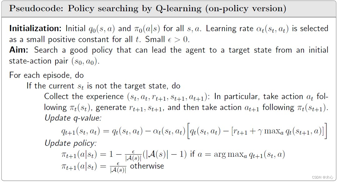
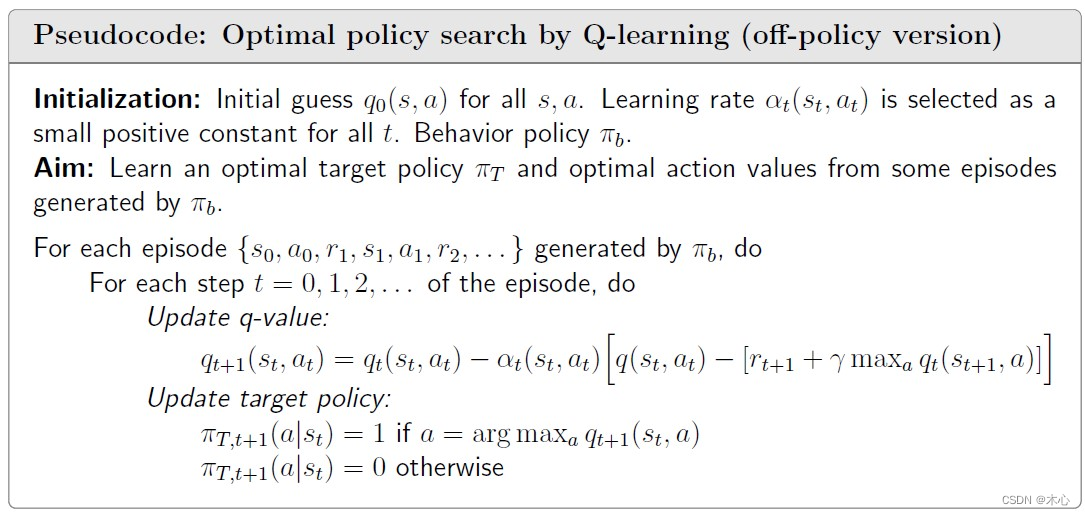
Persudocode:
(On-policy version)
(Off-policy version)
Reference
赵世钰老师的课程


![[数据库]对数据库事务进行总结](https://img-blog.csdnimg.cn/84a35a874e954e4da9d0050ba933d31b.png)