在【机器学习6】这篇文章中,笔者已经介绍过环境准备相关事项,本文对此不再赘述。本文将通过编程案例来探索特征组合(Feature Crosses)对模型训练的影响,加深对上一篇文章(机器学习8)的理解。
经度和纬度可以作为独立特征训练模型以预测当地房价。同时,我们也可以将经度和纬度进行交叉生成交叉特征,进而训练房价预测模型。那么,那种方式更好呢?更进一步,房价与精确的精度和纬度强相关么?未必,那么直接使用精度和纬度数据是不是不太合适呢?学习本篇文章,我们一起来探索吧。
目录
1.导入依赖
2.加载、缩放和打乱示例
3.将纬度和经度表示为浮点值
4.定义用于创建和训练模型的函数以及打印函数
5.用浮点表示法训练模型
6.完整代码运行
7.以桶表示纬度和经度
7.1 完整代码
7.2 运行结果
8.用特征交叉来表示位置
8.1 完整代码
8.2 运行结果
1.导入依赖
import numpy as np
import pandas as pd
import tensorflow as tf
from tensorflow.keras import layers
from matplotlib import pyplot as plt
2.加载、缩放和打乱示例
既然要训练模型,那就必须要有示例数据,因此,通过如下代码单元加载单独的 .csv 文件并创建两个数据集:
- train_df,训练数据集
- test_df,测试数据集
然后,将 median_house_value 缩放到更人性化的范围,然后对示例进行打乱。
# 载入数据集
train_df = pd.read_csv("https://download.mlcc.google.com/mledu-datasets/california_housing_train.csv")
test_df = pd.read_csv("https://download.mlcc.google.com/mledu-datasets/california_housing_test.csv")

# 缩放标签
scale_factor = 1000.0
# 缩放训练集的标签
train_df["median_house_value"] /= scale_factor

# 缩放测试集的标签
test_df["median_house_value"] /= scale_factor

# 打乱示例
train_df = train_df.reindex(np.random.permutation(train_df.index))
3.将纬度和经度表示为浮点值
在【机器学习6】中,我们训练线性回归模型只用到了单一特征。相比之下,这里我们将使用输入层训练两个特征。
社区的位置通常是决定房屋价值的最重要特征。加州住房数据集提供了两个特征,即纬度和经度,用于识别每个社区的位置。
下面的代码单元定义了两个 tf.keras.Input 层,一个表示纬度,另一个表示经度,都是浮点值。这个代码单元指定了用于训练模型的特征,以及这些特征将如何表示。
# 通过 Keras(一个由 Python 编写的开源人工神经网络库)将经度和纬度浮点值的输入张量
inputs = {
    'latitude':
        tf.keras.layers.Input(shape=(1,), dtype=tf.float32,
                              name='latitude'),
    'longitude':
        tf.keras.layers.Input(shape=(1,), dtype=tf.float32,
                              name='longitude')
}
4.定义用于创建和训练模型的函数以及打印函数
以下代码定义了三个功能:
- create_model,它告诉 TensorFlow 根据提供的输入和输出构建线性回归模型。
- train_model,它将基于训练集中的示例训练模型。
- plot_the_loss_curve,生成损失曲线。
# 创建模型
def create_model(my_inputs, my_outputs, my_learning_rate):
    model = tf.keras.Model(inputs=my_inputs, outputs=my_outputs)

    # 将层编译为 TensorFlow 可以执行的模型
    model.compile(optimizer=tf.keras.optimizers.experimental.RMSprop(
        learning_rate=my_learning_rate),
        loss="mean_squared_error",
        metrics=[tf.keras.metrics.RootMeanSquaredError()])

    return model


# 训练模型
def train_model(model, dataset, epochs, batch_size, label_name):
    # 将数据集输入到模型中以便对其进行训练
    features = {name: np.array(value) for name, value in dataset.items()}
    label = np.array(features.pop(label_name))
    history = model.fit(x=features, y=label, batch_size=batch_size,
                        epochs=epochs, shuffle=True)

    # 将轮次列表与历史的其余部分分开存储
    epochs = history.epoch

    # 隔离每一轮训练的平均绝对误差
    hist = pd.DataFrame(history.history)
    rmse = hist["root_mean_squared_error"]

    return epochs, rmse


# 打印损失
def plot_the_loss_curve(epochs, rmse):
    # 绘制损失与训练轮次的曲线
    plt.figure()
    plt.xlabel("Epoch")
    plt.ylabel("Root Mean Squared Error")

    plt.plot(epochs, rmse, label="Loss")
    plt.legend()
    plt.ylim([rmse.min() * 0.94, rmse.max() * 1.05])
    plt.show()
5.用浮点表示法训练模型
执行下面的代码单元来训练、绘制和评估模型。
# 初始化超参数
learning_rate = 0.05
epochs = 30
batch_size = 100
label_name = 'median_house_value'

# 将两个输入层连接在一起,以便将它们作为单个张量传递到密集层
preprocessing_layer = tf.keras.layers.Concatenate()(inputs.values())

dense_output = layers.Dense(
    units=1,
    input_shape=(1,),
    name='dense_layer')(preprocessing_layer)

outputs = {
    'dense_output': dense_output
}

# 创建并编译模型
my_model = create_model(inputs, outputs, learning_rate)

# 基于训练数据集训练模型
epochs, rmse = train_model(my_model, train_df, epochs, batch_size, label_name)

# 打印出模型摘要
my_model.summary(expand_nested=True)

plot_the_loss_curve(epochs, rmse)

print("\n: Evaluate the new model against the test set:")
test_features = {name: np.array(value) for name, value in test_df.items()}
test_label = np.array(test_features.pop(label_name))
my_model.evaluate(x=test_features, y=test_label, batch_size=batch_size)
6.完整代码运行
将上面的代码整合到一起,可以得到如下代码:
import numpy as np
import pandas as pd
import tensorflow as tf
from tensorflow.keras import layers
from matplotlib import pyplot as plt

pd.options.display.max_rows = 10
pd.options.display.float_format = "{:.1f}".format

tf.keras.backend.set_floatx('float32')

print("Imported the modules.")

# 载入数据集(注意:这里已经将谷歌的原始数据文件下载到了本地,因此用的是本地路径)
train_df = pd.read_csv("/Users/jinKwok/Downloads/california_housing_train.csv")
test_df = pd.read_csv("/Users/jinKwok/Downloads/california_housing_test.csv")

# 缩放标签
scale_factor = 1000.0
# 缩放训练集的标签
train_df["median_house_value"] /= scale_factor

# 缩放测试集的标签
test_df["median_house_value"] /= scale_factor

# 打乱示例
train_df = train_df.reindex(np.random.permutation(train_df.index))

# 通过 Keras(一个由 Python 编写的开源人工神经网络库)将经度和纬度浮点值的输入张量
inputs = {
    'latitude':
        tf.keras.layers.Input(shape=(1,), dtype=tf.float32,
                              name='latitude'),
    'longitude':
        tf.keras.layers.Input(shape=(1,), dtype=tf.float32,
                              name='longitude')
}


# 创建模型
def create_model(my_inputs, my_outputs, my_learning_rate):
    model = tf.keras.Model(inputs=my_inputs, outputs=my_outputs)

    # 将层编译为 TensorFlow 可以执行的模型
    model.compile(optimizer=tf.keras.optimizers.experimental.RMSprop(
        learning_rate=my_learning_rate),
        loss="mean_squared_error",
        metrics=[tf.keras.metrics.RootMeanSquaredError()])

    return model


# 训练模型
def train_model(model, dataset, epochs, batch_size, label_name):
    # 将数据集输入到模型中以便对其进行训练
    features = {name: np.array(value) for name, value in dataset.items()}
    label = np.array(features.pop(label_name))
    history = model.fit(x=features, y=label, batch_size=batch_size,
                        epochs=epochs, shuffle=True)

    # 将轮次列表与历史的其余部分分开存储
    epochs = history.epoch

    # 隔离每一轮训练的平均绝对误差
    hist = pd.DataFrame(history.history)
    rmse = hist["root_mean_squared_error"]

    return epochs, rmse


# 打印损失
def plot_the_loss_curve(epochs, rmse):
    # 绘制损失与训练轮次的曲线
    plt.figure()
    plt.xlabel("Epoch")
    plt.ylabel("Root Mean Squared Error")

    plt.plot(epochs, rmse, label="Loss")
    plt.legend()
    plt.ylim([rmse.min() * 0.94, rmse.max() * 1.05])
    plt.show()


print("Defined the create_model, train_model, and plot_the_loss_curve functions.")

# 初始化超参数
learning_rate = 0.05
epochs = 30
batch_size = 100
label_name = 'median_house_value'

# 将两个输入层连接在一起,以便将它们作为单个张量传递到密集层
preprocessing_layer = tf.keras.layers.Concatenate()(inputs.values())

dense_output = layers.Dense(
    units=1,
    input_shape=(1,),
    name='dense_layer')(preprocessing_layer)

outputs = {
    'dense_output': dense_output
}

# 创建并编译模型
my_model = create_model(inputs, outputs, learning_rate)

# 基于训练数据集训练模型
epochs, rmse = train_model(my_model, train_df, epochs, batch_size, label_name)

# 打印出模型摘要
my_model.summary(expand_nested=True)

plot_the_loss_curve(epochs, rmse)

print("\n: Evaluate the new model against the test set:")
test_features = {name: np.array(value) for name, value in test_df.items()}
test_label = np.array(test_features.pop(label_name))
my_model.evaluate(x=test_features, y=test_label, batch_size=batch_size)
运行结果如下所示:
_________________________________________________________________________________________________
 Layer (type)                   Output Shape         Param #     Connected to
==================================================================================================
 latitude (InputLayer)          [(None, 1)]          0           []

 longitude (InputLayer)         [(None, 1)]          0           []

 concatenate (Concatenate)      (None, 2)            0           ['latitude[0][0]',
                                                                  'longitude[0][0]']

 dense_layer (Dense)            (None, 1)            3           ['concatenate[0][0]']

==================================================================================================
Total params: 3
Trainable params: 3
Non-trainable params: 0
__________________________________________________________________________________________________
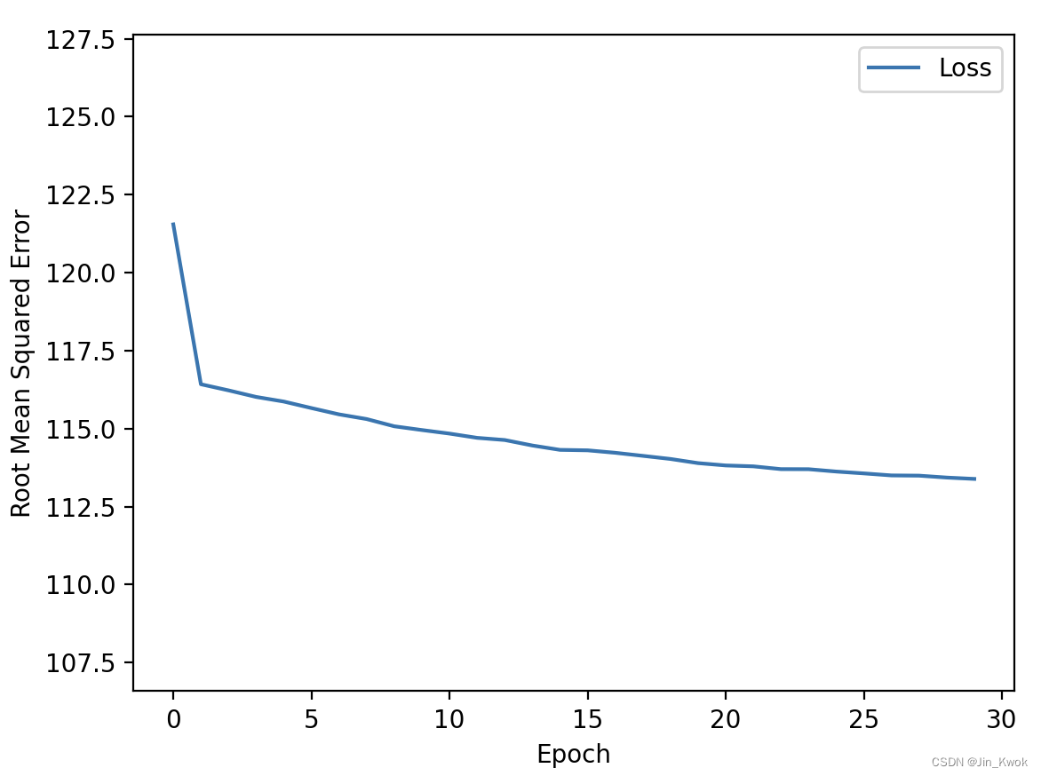
从上面的损失曲线来看,训练并没有收敛,这说明用浮点值表示纬度和经度并不合适。鉴于此,我们继续尝试其他方法。
7.以桶表示纬度和经度
以下图所示,我们用 “桶” 来表示经度和纬度。每个 “桶” 表示一个区间内的所有邻域,例如,纬度 32.4 和 32.8 的邻域在同一个桶(LatitudeBin1)中,但纬度 37.4 与 38.2 的邻域在不同的桶中。

模型将学习每个 “桶” 的权重。例如,模型将为 “LatitudeBin1” 桶学习一个权重,为 “LatitudeBin2” 桶学习另一个不同的权重,依此类推,此表示将创建大约 20 个桶。
- 纬度为 10 个桶
- 经度为 10 个桶
相关代码如下:
resolution_in_degrees = 1.0

# 创建一个数字列表,用来表示纬度的桶边界,简单理解就是确定纬度分组的数据段
latitude_boundaries = list(np.arange(int(min(train_df['latitude'])),
                                     int(max(train_df['latitude'])),
                                     resolution_in_degrees))
print("latitude boundaries: " + str(latitude_boundaries))

# 创建一个离散化层,将纬度数据分离存储到桶中
latitude = tf.keras.layers.Discretization(
    bin_boundaries=latitude_boundaries,
    name='discretization_latitude')(inputs.get('latitude'))

# 纬度类别数量 = 纬度边界数量 + 1,这很好理解,比如对一根香肠划5刀,可以将其分为6段
latitude = tf.keras.layers.CategoryEncoding(
    num_tokens=len(latitude_boundaries) + 1,
    output_mode='one_hot',
    name='category_encoding_latitude')(latitude)

# 创建一个数字列表,用来表示经度的桶边界
longitude_boundaries = list(np.arange(int(min(train_df['longitude'])),
                                      int(max(train_df['longitude'])),
                                      resolution_in_degrees))

print("longitude boundaries: " + str(longitude_boundaries))

# 创建一个离散化层,将经度数据分离存储到桶中
longitude = tf.keras.layers.Discretization(
    bin_boundaries=longitude_boundaries,
    name='discretization_longitude')(inputs.get('longitude'))

# 经度类别数量 = 经度边界数量 + 1,这很好理解,比如对一根香肠划5刀,可以将其分为6段
longitude = tf.keras.layers.CategoryEncoding(
    num_tokens=len(longitude_boundaries) + 1,
    output_mode='one_hot',
    name='category_encoding_longitude')(longitude)

# 将纬度和经度连接到单个张量中,作为密集层的输入。
concatenate_layer = tf.keras.layers.Concatenate()([latitude, longitude])

dense_output = layers.Dense(
    units=1, input_shape=(2,), name='dense_layer')(concatenate_layer)

# 定义一个输出字典,我们将发送给模型构造函数
outputs = {
    'dense_output': dense_output
}
7.1 完整代码
将上面的代码整合到完整的工程中。需要注意的是:google提供的原始数据地址为:https://download.mlcc.google.com/mledu-datasets/california_housing_train.csv
https://download.mlcc.google.com/mledu-datasets/california_housing_test.csv
为了便于本地执行,我们将数据下载到了本地,读者如果要运行代码,将程序中的数据路径修改为自己的数据路径即可。
import numpy as np
import pandas as pd
import tensorflow as tf
from tensorflow.keras import layers
from matplotlib import pyplot as plt

pd.options.display.max_rows = 10
pd.options.display.float_format = "{:.1f}".format

tf.keras.backend.set_floatx('float32')

print("Imported the modules.")

# 载入数据集,谷歌原始数据访问太慢了,这里我们将数据下载的到本地,因此使用的是本地路径
train_df = pd.read_csv("/Users/jinKwok/Downloads/california_housing_train.csv")
test_df = pd.read_csv("/Users/jinKwok/Downloads/california_housing_test.csv")

# 缩放标签
scale_factor = 1000.0
# 缩放训练集的标签
train_df["median_house_value"] /= scale_factor

# 缩放测试集的标签
test_df["median_house_value"] /= scale_factor

# 打乱示例
train_df = train_df.reindex(np.random.permutation(train_df.index))

# 通过 Keras(一个由 Python 编写的开源人工神经网络库)将经度和纬度浮点值的输入张量
inputs = {
    'latitude':
        tf.keras.layers.Input(shape=(1,), dtype=tf.float32,
                              name='latitude'),
    'longitude':
        tf.keras.layers.Input(shape=(1,), dtype=tf.float32,
                              name='longitude')
}


# 创建模型
def create_model(my_inputs, my_outputs, my_learning_rate):
    model = tf.keras.Model(inputs=my_inputs, outputs=my_outputs)

    # 将层编译为 TensorFlow 可以执行的模型
    model.compile(optimizer=tf.keras.optimizers.experimental.RMSprop(
        learning_rate=my_learning_rate),
        loss="mean_squared_error",
        metrics=[tf.keras.metrics.RootMeanSquaredError()])

    return model


# 训练模型
def train_model(model, dataset, epochs, batch_size, label_name):
    # 将数据集输入到模型中以便对其进行训练
    features = {name: np.array(value) for name, value in dataset.items()}
    label = np.array(features.pop(label_name))
    history = model.fit(x=features, y=label, batch_size=batch_size,
                        epochs=epochs, shuffle=True)

    # 将轮次列表与历史的其余部分分开存储
    epochs = history.epoch

    # 隔离每一轮训练的平均绝对误差
    hist = pd.DataFrame(history.history)
    rmse = hist["root_mean_squared_error"]

    return epochs, rmse


# 打印损失
def plot_the_loss_curve(epochs, rmse):
    # 绘制损失与训练轮次的曲线
    plt.figure()
    plt.xlabel("Epoch")
    plt.ylabel("Root Mean Squared Error")

    plt.plot(epochs, rmse, label="Loss")
    plt.legend()
    plt.ylim([rmse.min() * 0.94, rmse.max() * 1.05])
    plt.show()


print("Defined the create_model, train_model, and plot_the_loss_curve functions.")

# 初始化超参数
learning_rate = 0.05
epochs = 30
batch_size = 100
label_name = 'median_house_value'

#################################
resolution_in_degrees = 1.0

# 创建一个数字列表,用来表示纬度的桶边界,简单理解就是确定纬度分组的数据段
latitude_boundaries = list(np.arange(int(min(train_df['latitude'])),
                                     int(max(train_df['latitude'])),
                                     resolution_in_degrees))
print("latitude boundaries: " + str(latitude_boundaries))

# 创建一个离散化层,将纬度数据分离存储到桶中
latitude = tf.keras.layers.Discretization(
    bin_boundaries=latitude_boundaries,
    name='discretization_latitude')(inputs.get('latitude'))

# 纬度类别数量 = 纬度边界数量 + 1,这很好理解,比如对一根香肠划5刀,可以将其分为6段
latitude = tf.keras.layers.CategoryEncoding(
    num_tokens=len(latitude_boundaries) + 1,
    output_mode='one_hot',
    name='category_encoding_latitude')(latitude)

# 创建一个数字列表,用来表示经度的桶边界
longitude_boundaries = list(np.arange(int(min(train_df['longitude'])),
                                      int(max(train_df['longitude'])),
                                      resolution_in_degrees))

print("longitude boundaries: " + str(longitude_boundaries))

# 创建一个离散化层,将经度数据分离存储到桶中
longitude = tf.keras.layers.Discretization(
    bin_boundaries=longitude_boundaries,
    name='discretization_longitude')(inputs.get('longitude'))

# 经度类别数量 = 经度边界数量 + 1,这很好理解,比如对一根香肠划5刀,可以将其分为6段
longitude = tf.keras.layers.CategoryEncoding(
    num_tokens=len(longitude_boundaries) + 1,
    output_mode='one_hot',
    name='category_encoding_longitude')(longitude)

# 将纬度和经度连接到单个张量中,作为密集层的输入。
concatenate_layer = tf.keras.layers.Concatenate()([latitude, longitude])

dense_output = layers.Dense(
    units=1, input_shape=(2,), name='dense_layer')(concatenate_layer)

# 定义一个输出字典,我们将发送给模型构造函数
outputs = {
    'dense_output': dense_output
}

# 创建并编译模型
my_model = create_model(inputs, outputs, learning_rate)

# 基于训练数据集训练模型
epochs, rmse = train_model(my_model, train_df, epochs, batch_size, label_name)

# 打印出模型摘要
my_model.summary(expand_nested=True)

plot_the_loss_curve(epochs, rmse)

print("\n: Evaluate the new model against the test set:")
test_features = {name: np.array(value) for name, value in test_df.items()}
test_label = np.array(test_features.pop(label_name))
my_model.evaluate(x=test_features, y=test_label, batch_size=batch_size)
7.2 运行结果
__________________________________________________________________________________________________
 Layer (type)                   Output Shape         Param #     Connected to
==================================================================================================
 latitude (InputLayer)          [(None, 1)]          0           []

 longitude (InputLayer)         [(None, 1)]          0           []

 discretization_latitude (Discr  (None, 1)           0           ['latitude[0][0]']
 etization)

 discretization_longitude (Disc  (None, 1)           0           ['longitude[0][0]']
 retization)

 category_encoding_latitude (Ca  (None, 10)          0           ['discretization_latitude[0][0]']
 tegoryEncoding)

 category_encoding_longitude (C  (None, 11)          0           ['discretization_longitude[0][0]'
 ategoryEncoding)                                                ]

 concatenate (Concatenate)      (None, 21)           0           ['category_encoding_latitude[0][0
                                                                 ]',
                                                                  'category_encoding_longitude[0][
                                                                 0]']

 dense_layer (Dense)            (None, 1)            22          ['concatenate[0][0]']

==================================================================================================
Total params: 22
Trainable params: 22
Non-trainable params: 0
__________________________________________________________________________________________________
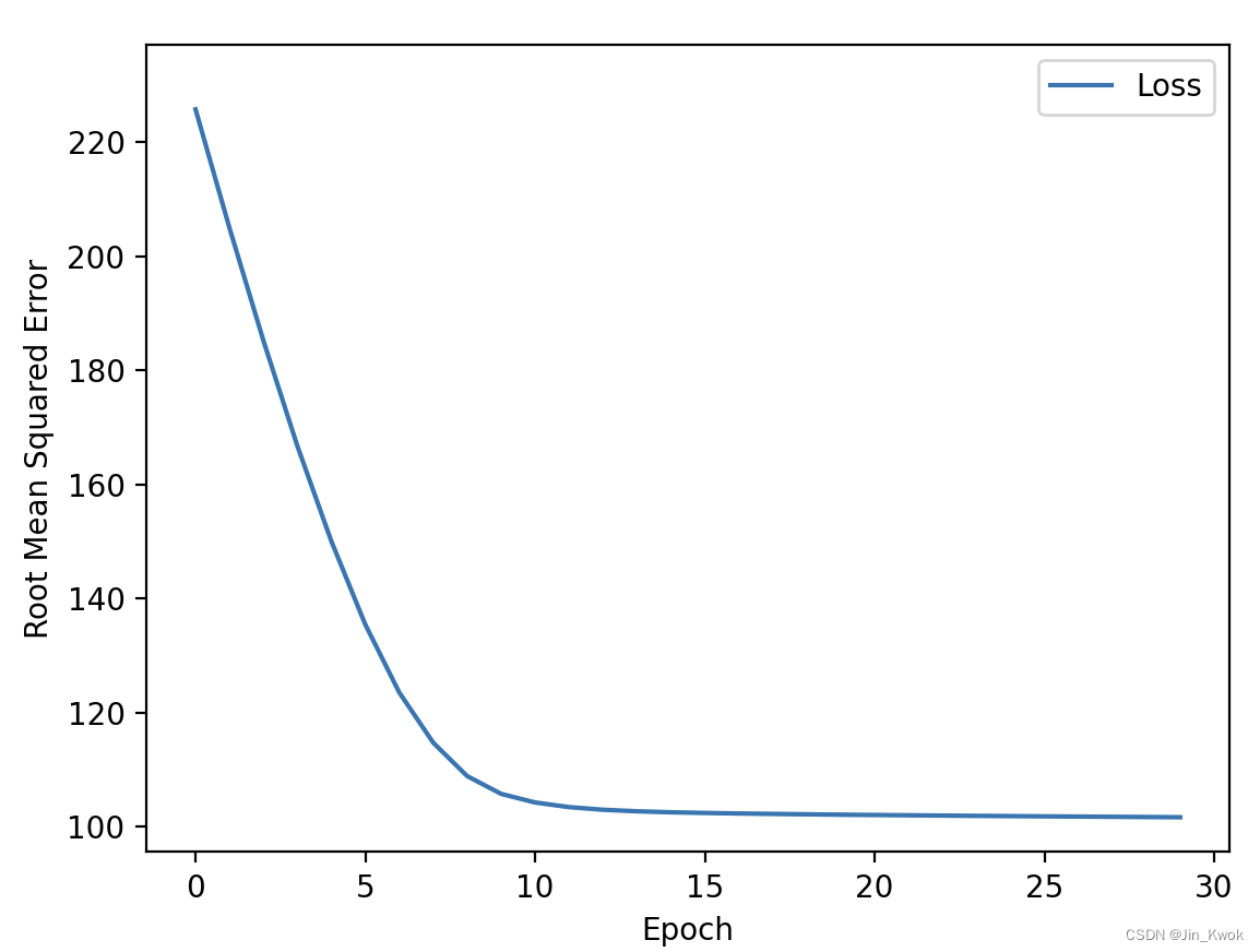
从损失曲线来看,相较于用浮点表示法训练模型,用桶表示纬度和经度的收敛效果要好的多。
8.用特征交叉来表示位置
如下代码所示,将位置表示为交叉特征。也就是说,下面的代码单元首先创建 bucket,然后使用HashedCrossing 层交叉纬度和经度特性。
resolution_in_degrees = 1.0

# 创建一个数字列表,用来表示纬度的桶边界,简单理解就是确定纬度分组的数据段
latitude_boundaries = list(np.arange(int(min(train_df['latitude'])),
                                     int(max(train_df['latitude'])),
                                     resolution_in_degrees))
print("latitude boundaries: " + str(latitude_boundaries))

# 创建一个离散化层,将纬度数据分离存储到桶中
latitude = tf.keras.layers.Discretization(
    bin_boundaries=latitude_boundaries,
    name='discretization_latitude')(inputs.get('latitude'))

# 创建一个数字列表,用来表示经度的桶边界
longitude_boundaries = list(np.arange(int(min(train_df['longitude'])),
                                      int(max(train_df['longitude'])),
                                      resolution_in_degrees))

print("longitude boundaries: " + str(longitude_boundaries))

# 创建一个离散化层,将经度数据分离存储到桶中
longitude = tf.keras.layers.Discretization(
    bin_boundaries=longitude_boundaries,
    name='discretization_longitude')(inputs.get('longitude'))

# 将纬度和经度特征交叉成一个单一的热向量
feature_cross = tf.keras.layers.HashedCrossing(
    num_bins=len(latitude_boundaries) * len(longitude_boundaries),
    output_mode='one_hot',
    name='cross_latitude_longitude')([latitude, longitude])

dense_output = layers.Dense(units=1, input_shape=(2,),
                            name='dense_layer')(feature_cross)

# 定义一个输出字典,我们将发送给模型构造函数
outputs = {
    'dense_output': dense_output
}
8.1 完整代码
将上面的代码整合到完整的工程中,得到如下所示的完整代码,读者修改其中的数据文件路径后,可在本地直接运行。
import numpy as np
import pandas as pd
import tensorflow as tf
from tensorflow.keras import layers
from matplotlib import pyplot as plt

pd.options.display.max_rows = 10
pd.options.display.float_format = "{:.1f}".format

tf.keras.backend.set_floatx('float32')

print("Imported the modules.")

# 载入数据集
train_df = pd.read_csv("/Users/jinKwok/Downloads/california_housing_train.csv")
test_df = pd.read_csv("/Users/jinKwok/Downloads/california_housing_test.csv")

# 缩放标签
scale_factor = 1000.0
# 缩放训练集的标签
train_df["median_house_value"] /= scale_factor

# 缩放测试集的标签
test_df["median_house_value"] /= scale_factor

# 打乱示例
train_df = train_df.reindex(np.random.permutation(train_df.index))

# 通过 Keras(一个由 Python 编写的开源人工神经网络库)将经度和纬度浮点值的输入张量
inputs = {
    'latitude':
        tf.keras.layers.Input(shape=(1,), dtype=tf.float32,
                              name='latitude'),
    'longitude':
        tf.keras.layers.Input(shape=(1,), dtype=tf.float32,
                              name='longitude')
}


# 创建模型
def create_model(my_inputs, my_outputs, my_learning_rate):
    model = tf.keras.Model(inputs=my_inputs, outputs=my_outputs)

    # 将层编译为 TensorFlow 可以执行的模型
    model.compile(optimizer=tf.keras.optimizers.experimental.RMSprop(
        learning_rate=my_learning_rate),
        loss="mean_squared_error",
        metrics=[tf.keras.metrics.RootMeanSquaredError()])

    return model


# 训练模型
def train_model(model, dataset, epochs, batch_size, label_name):
    # 将数据集输入到模型中以便对其进行训练
    features = {name: np.array(value) for name, value in dataset.items()}
    label = np.array(features.pop(label_name))
    history = model.fit(x=features, y=label, batch_size=batch_size,
                        epochs=epochs, shuffle=True)

    # 将轮次列表与历史的其余部分分开存储
    epochs = history.epoch

    # 隔离每一轮训练的平均绝对误差
    hist = pd.DataFrame(history.history)
    rmse = hist["root_mean_squared_error"]

    return epochs, rmse


# 打印损失
def plot_the_loss_curve(epochs, rmse):
    # 绘制损失与训练轮次的曲线
    plt.figure()
    plt.xlabel("Epoch")
    plt.ylabel("Root Mean Squared Error")

    plt.plot(epochs, rmse, label="Loss")
    plt.legend()
    plt.ylim([rmse.min() * 0.94, rmse.max() * 1.05])
    plt.show()


print("Defined the create_model, train_model, and plot_the_loss_curve functions.")

# 初始化超参数
learning_rate = 0.04
epochs = 35
batch_size = 100
label_name = 'median_house_value'

#################################
resolution_in_degrees = 1.0

# 创建一个数字列表,用来表示纬度的桶边界,简单理解就是确定纬度分组的数据段
latitude_boundaries = list(np.arange(int(min(train_df['latitude'])),
                                     int(max(train_df['latitude'])),
                                     resolution_in_degrees))
print("latitude boundaries: " + str(latitude_boundaries))

# 创建一个离散化层,将纬度数据分离存储到桶中
latitude = tf.keras.layers.Discretization(
    bin_boundaries=latitude_boundaries,
    name='discretization_latitude')(inputs.get('latitude'))

# 创建一个数字列表,用来表示经度的桶边界
longitude_boundaries = list(np.arange(int(min(train_df['longitude'])),
                                      int(max(train_df['longitude'])),
                                      resolution_in_degrees))

print("longitude boundaries: " + str(longitude_boundaries))

# 创建一个离散化层,将经度数据分离存储到桶中
longitude = tf.keras.layers.Discretization(
    bin_boundaries=longitude_boundaries,
    name='discretization_longitude')(inputs.get('longitude'))

# 将纬度和经度特征交叉成一个单一的热向量
feature_cross = tf.keras.layers.HashedCrossing(
    num_bins=len(latitude_boundaries) * len(longitude_boundaries),
    output_mode='one_hot',
    name='cross_latitude_longitude')([latitude, longitude])

dense_output = layers.Dense(units=1, input_shape=(2,),
                            name='dense_layer')(feature_cross)

# 定义一个输出字典,我们将发送给模型构造函数
outputs = {
    'dense_output': dense_output
}

# 创建并编译模型
my_model = create_model(inputs, outputs, learning_rate)

# 基于训练数据集训练模型
epochs, rmse = train_model(my_model, train_df, epochs, batch_size, label_name)

# 打印出模型摘要
my_model.summary(expand_nested=True)

plot_the_loss_curve(epochs, rmse)

print("\n: Evaluate the new model against the test set:")
test_features = {name: np.array(value) for name, value in test_df.items()}
test_label = np.array(test_features.pop(label_name))
my_model.evaluate(x=test_features, y=test_label, batch_size=batch_size)
8.2 运行结果
__________________________________________________________________________________________________
 Layer (type)                   Output Shape         Param #     Connected to
==================================================================================================
 latitude (InputLayer)          [(None, 1)]          0           []

 longitude (InputLayer)         [(None, 1)]          0           []

 discretization_latitude (Discr  (None, 1)           0           ['latitude[0][0]']
 etization)

 discretization_longitude (Disc  (None, 1)           0           ['longitude[0][0]']
 retization)

 cross_latitude_longitude (Hash  (None, 90)          0           ['discretization_latitude[0][0]',
 edCrossing)                                                      'discretization_longitude[0][0]'
                                                                 ]

 dense_layer (Dense)            (None, 1)            91          ['cross_latitude_longitude[0][0]'
                                                                 ]

==================================================================================================
Total params: 91
Trainable params: 91
Non-trainable params: 0
__________________________________________________________________________________________________
从损失曲线来看, 用特征交叉来表示位置训练模型,其 “root_mean_squared_error” 要更小一些,这也说明,在本案例中,交叉特征能够产生更好的效果。