NeRF与三维重建专栏（三）nerf_pl源码部分解读与colmap、cuda算子使用

前言上一章中我们介绍了NeRF原理、传统体渲染方法以及两者之间的联系，本章中我们将讲解colmap的安装以及使用，部分nerf_pl源码，同时在开发过程中，由于部分操作python/torch不支持，我们需要自己造轮子，且在后续的专栏中我们也会遇到cuda算子，因此本章也会讲解一下cuda算子的使用。

本教程禁止转载。同时，本教程来自知识星球【CV技术指南】更多技术教程，可加入星球学习。

Transformer、目标检测、语义分割交流群

欢迎关注公众号CV技术指南，专注于计算机视觉的技术总结、最新技术跟踪、经典论文解读、CV招聘信息。

CV各大方向专栏与各个部署框架最全教程整理

colmap安装与使用

colmp是一个基于C++的开源计算机视觉库，提供多个工具用于三维重建、图像检索、结构从运动估计、2D/3D特征提取与匹配等任务。它的目标是提供一个功能强大，灵活且易于使用的平台，以促进学术研究、教育和产品开发。Colmap的特点是可以使用CPU或GPU进行计算，支持多种图像格式和相机模型，以及提供了多种数据集导入和导出格式。

由于本专栏主要关注NeRF with pose，因此我们首先需要知道如何获得相机位姿。

1.下载colmap并编译：

colmp源码下载地址，选择最新的版本tag，然后我们根据其document的流程编译即可

网上还有很多其他colmap编译安装教程，因为环境等问题遇到的bug我们这里就不赘述如何解决了

2.使用colmap

其实网上已经有很多colmap的示例教程了，这里我们简要介绍一下colmap gui的使用：

在bash中输入colmap gui，得到gui界面：

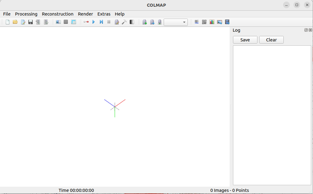
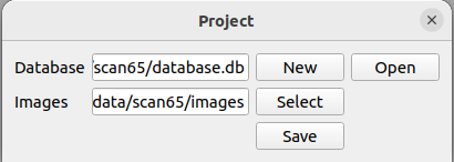
在file中选择new project，在Database中选择New，新建一个database.db（不需要自己手动建，在输入栏中输入database.db可以自动新建）；在images栏中选择图像目录（可以有子目录，但图像目录下所有子目录的图片都应该是拍摄同一个场景的），选择save；

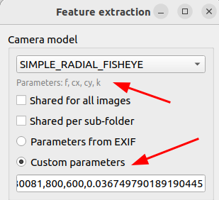
然后选择processing中的feature extraction，如果不知道相机内参，直接点击extract即可，如果有内参，我们可以选择custom parameters，然后依次输入相机的内参（内参表会根据你选择不同的相机模型而不同，一般焦距准确了重建效果不会太差）：

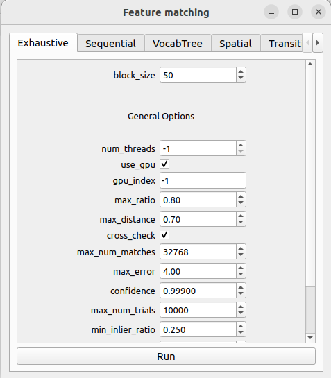
特征提取结束后进入匹配，选择processing中的feature matching，如果有词汇树，可以导入词汇树文件；如果是连续帧，可以选择Sequential并限定相邻帧的数目上限；都不是可以选择Exhaustive，也即暴力匹配（小场景下不会花费多少时间）

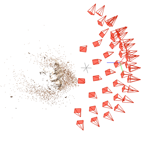
匹配后选择Reconstruction中的start reconstruction，即可开始稀疏重建，得到重建结果：

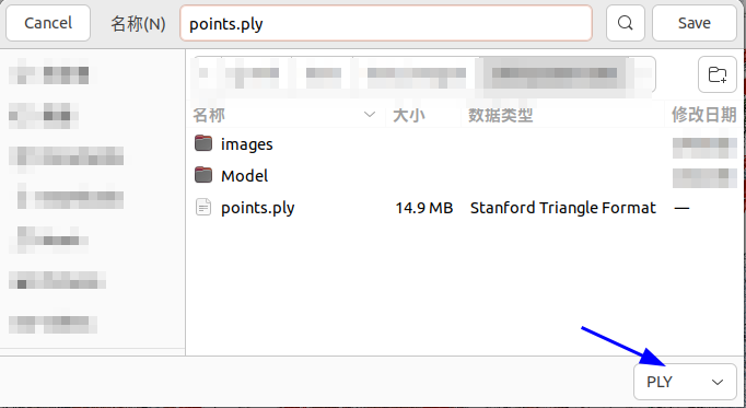
然后我们可以选择files中的export model，我们可以选择将cameras、images、points3D输出为bin或者txt格式，其中cameras中存放的是相机的内参，images中存放了每幅图片的名字、位姿（以四元数方式存储）、特征点描述子，points文件中存放了稀疏点云相关信息（如果想要ply格式，可以选择file中的export model as ...，在右下方选择``PLY```）

cuda算子

由于部分操作在python不支持，或是因为torch/多线程相对于GPU运算更慢，我们有时需要自己写一些cuda算子。例如在nerf类方法中经常用到的ray marhing算法，或者图形学中的aabb intersection检测。但我们的目的不是成为轮子制造者，不需要对每一个能用cuda计算的操作都写一个cuda算子，学习cuda算子仅仅是为了我们实现想法多一种手段；同时我们也不需要深入了解cuda的一些进阶技巧例如数据对齐，使用纹理内存等，仅仅把它当作一个C++实现就好。请注意，这里我们假定读者已经装好了cuda。

1.GPU并行计算原理概述

在CPU单线程计算中，一个线程只能调用一份代码，一份代码只能处理一份数据，这意味着程序的计算能力被限制在一个CPU核心上；当我们不满足单线程的计算能力时，可以利用多个CPU核心来并行运行多个线程处理多份数据；

然而CPU多线程在同一时间段的计算上限只有仅仅几十个线程（这取决于你的内存大小和CPU型号），对比同时期的显卡，计算单元的数目可以相差三四个数量级，例如NVIDIA A2000的计算核心为3328，NVIDA 5000的计算核心为8192，这些计算核心分布在几十个流多处理器（SM，A2000为26，A5000为64）上，每个SM可以同时运行2048个线程。

而在cuda框架中，我们是如何来控制每一个线程的计算的呢？首先我们需要介绍cuda的两个抽象数据结构：block和thread

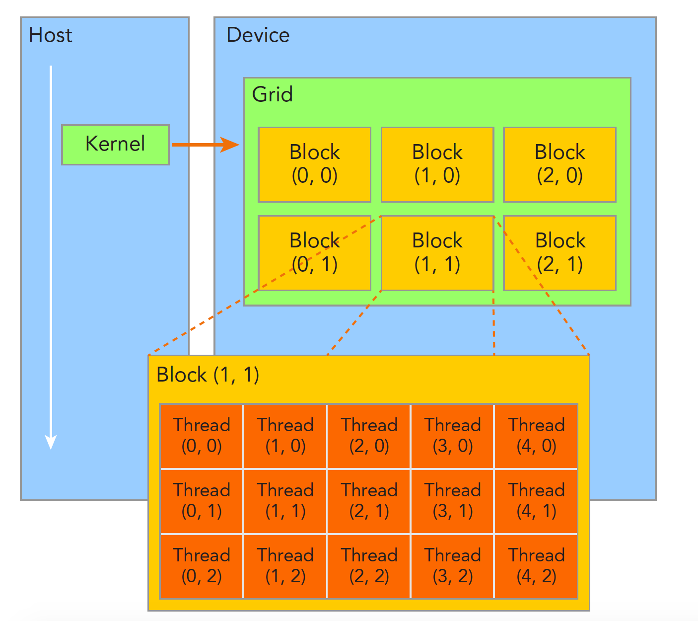
一个函数（kernel函数）可以调控一个Grid的计算资源，每个Grid可以自定义多个block，每个block上可以自定义多个thread（但block和thread并不是这样物理分布在GPU上的，它们仅仅是一种抽象数据结构），每个计算单元可以独立运行这个核函数，同时根据不同__线程的编号__处理不同的数据。例如我们可以建立线程编号到图像像素坐标的一一映射，从而让每个线程单独处理一个像素（例如求这个像素邻域的均值）。

我们可以通过内建变量threadIdx和blockIdx获取当前计算单元所在的block与所在的thread，其中blockIdx与threadIdx都是一个三元组，含有x，y，z成员变量，表示block所在grid的位置与thread所在block的位置（在cv领域，通常情况下我们不会用到z，仅用x，y足以覆盖整幅图像），例如：

// kernel
const int BLOCK_W = 64;
const int BLOCK_H = 16;
const dim3 blockSize(BLOCK_W,BLOCK_H,1);
const dim3 gridSize((num_pixs + BLOCK_W*BLOCK_H - 1)/(BLOCK_W * BLOCK_H),1,1);
// num_pixs = 500 * 300
...

上面的代码中，我们在kernel函数中声明了一个block的大小为 $64\times16$ ，而一个grid包含 $\frac{500\times300+64\times16-1}{64\times16}\approx147$ 个block，且这些block沿blockIdx.x方向呈一维线性排列；那么每一个线程的“绝对编号”就可以表示为：

// device
const int32_t n = blockIdx.x*blockDim.x*blockDim.y + threadIdx.x*blockDim.y + threadIdx.y

这里我们可以画一画block与thread的布局，以更好地理解：

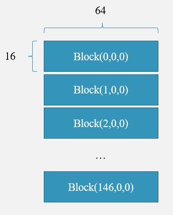
若有一个线程位于Block(2,0,0)，且其所在Block(2,0,0)的线程编号为thread(25,16,0)，则其编号为__当前block前面所有block的线程数__+所在当前block的线程编号，也即 $2\times16\times64+25\times16+16=2464$ ，这个数字表示该线程对应长为 $300\times500$ 向量中的第2465个元素。

想更深入的同学可以参考cuda官方文档。

2.cuda算子和pybinding

正常的cuda程序运行是需要nvcc编译器编译的，若在linux上我们还需要编写繁琐的CMakeLists，所幸我们使用的是pybinding，编译相关的操作我们可以交给python的setuptools库，同时将数据从内存拷贝到GPU上的操作可以用torch实现，我们不用了解cuda相对复杂的memcpy策略；唯一的缺点是不能调试所写的cuda算子。

但为了能够调试，我们后面也会放上c++的项目代码。

3.实例

光是文字描述太过抽象，我们现在实现一个简易的cuda程序：

在大场景的NeRF中，由于网络的学习容量有限，我们需要对场景进行分块；

假设场景被分为了 $4\times4$ 个子区域，每个子区域的子NeRF都需要用观测到这个区域的图像进行训练，但一副图像往往观察到不止一个区域，因此对于每一个子区域，我们需要计算所有图片观察到该区域的像素部分，并用mask来标记（例如mega-nerf的做法）；

对于一副 $m\times n$ 大小的mask图像，其数据类型为bool，虽然这已经是python中最小的数据类型（1字节），但是对于一张高分辨率的图像（例如 $5000\times3000$ 分辨率），存储这个mask所需的空间为： $\frac{5000\times3000}{1024^2}\approx14$ MB，那么假设有1000张图片，所有mask的存储空间约为 $14$ GB；在大场景NeRF中，对于每一个分块的子NeRF，我们都需要 $14$ GB的存储空间也就是 $14\times16=224$ GB，起码这对于笔者来说是不可忍受的，尤其是当我们想要测试不同分块策略的效果时。

那么我们如果将mask图像向量化为一个 $15000000$ 长度的一维向量，向量的每一个元素是1bit（注意不是byte），那么存储空间就可以由224G缩减为 $\frac{15000000\times16\times1000}{8\times1024^3}\approx28$ GB，这和1000幅RGB图像大小（大概11GB）在一个数量级。

但若是用python来实现这个过程会变得很慢，即使用上多线程时间也会很长，回顾一下cuda的原理，我们不妨用cuda算子的形式实现这个过程：

3.1 cu算子核心部分

#include <iostream>
#include <torch/extension.h>
#include <ATen/ATen.h>
#include <ATen/TensorAccessor.h>
#include <ATen/cuda/CUDAContext.h>

using namespace std;

__global__ void packbits_u32_kernel(
    torch::PackedTensorAccessor32<int32_t,1,torch::RestrictPtrTraits> idx_array,
    torch::PackedTensorAccessor64<int64_t,1,torch::RestrictPtrTraits> bits_array
){
    // const int32_t n = blockIdx.x * blockDim.x + threadIdx.x;//block为一维时
    const int32_t n = blockIdx.x*blockDim.x*blockDim.y + threadIdx.x*blockDim.y + threadIdx.y;//block为二维时
    if(n > bits_array.size(0))
        return;
    int mask_size = 32;
    if (n == bits_array.size(0))
        mask_size = idx_array.size(0) % 32;
    const int64_t flag = 1;
    for(int i = 0 ; i < mask_size ; i++){
        int32_t hit_pix = idx_array[n*32 + i];
        if (hit_pix > 0){
            bits_array[n] |= flag << i;
        }
    }
}


torch::Tensor packbits_u32_cu(
    torch::Tensor idx_array,
    torch::Tensor bits_array
){
    // 每个线程处理32位长数据即32个像素
    const int num_pixs = std::ceil(idx_array.size(0)/32);
    const int BLOCK_W = 64;
    const int BLOCK_H = 16;
    const dim3 blockSize(BLOCK_W,BLOCK_H,1);
    const dim3 gridSize((num_pixs + BLOCK_W*BLOCK_H - 1)/(BLOCK_W * BLOCK_H),1,1);

    AT_DISPATCH_ALL_TYPES(idx_array.type(),"packbits_u32_cu",
    ([&] {
        packbits_u32_kernel<<<gridSize, blockSize>>>(
            idx_array.packed_accessor32<int32_t,1,torch::RestrictPtrTraits>(),
            bits_array.packed_accessor64<int64_t,1,torch::RestrictPtrTraits>()
        );
    }));
    return bits_array;
}

include中，torch库来自libtorch（这里是cu111版本，可以从这里下载不同版本的libtorch）;ATen库是基础张量和数学运算库（属于libtorch的一个子库）

上述代码中，host端函数packbits_u32_cu接收了向量化后的mask图像idx_array，以及一个用于bit化的int64数组bits_array；并规划了该函数所调控grid的block、thread布局；

然后通过AT_DISPATCH_ALL_TYPES将数据传入device端函数packbits_u32_kernel。

AT_DISPATCH_ALL_TYPES用于自动分派不同数据类型的张量到不同的函数中，其需要传入三个参数：数据类型d、函数名和函数参数列表；

[&]是c++中的一种lambda表达式，上述代码中[&]将其后的代码块打包为一个lambda函数，&表示该函数的所有变量以引用的方式传递；

<<< >>>是cuda中用来定义函数执行配置的符号，其左为device端函数，中为grid、block配置，右为参数列表。

而在packbits_u32_kernel中，每个线程截取idx_array的32个元素，并按照位运算赋值给bits_array中一个元素的32位，完成数据的缩减（这里我们采用int64而不是uint32，是因为ATen不支持uint32以及uint64）。

如果读者想了解更多，可以查阅torch的官方文档或直接查阅libtorch的api文档。笔者认为更容易上手的另一个例子是kwea123的三线性插值教程，该作者的cuda extension系列教程也适合大部分新手进一步学习。

那么cuda算子的核心部分已经完成，我们下面介绍如何使用python调用这个算子。

3.2 pybinding

通常我们在跨语言编程时，使用A语言调用B语言程序，需要将B语言的代码先打包为一个动态库。pybinding也不例外，我们首先需要构建完整的cuda源码，然后才能打包为动态库，此时我们的项目至少需要三个文件：头文件、binding.cpp、main.cu：

utils.h头文件：

#include <torch/extension.h>

#define CHECK_CUDA(x) TORCH_CHECK(x.is_cuda(), #x " must be a CUDA tensor")
#define CHECK_CONTIGUOUS(x) TORCH_CHECK(x.is_contiguous(), #x " must be contiguous")
#define CHECK_INPUT(x) CHECK_CUDA(x); CHECK_CONTIGUOUS(x)

torch::Tensor packbits_u32(torch::Tensor idx_array, torch::Tensor bits_array);

torch::Tensor un_packbits_u32(torch::Tensor idx_array, torch::Tensor bits_array);

torch::Tensor packbits_u32_cu(
    torch::Tensor idx_array,
    torch::Tensor bits_array
);

torch::Tensor un_packbits_u32_cu(
    torch::Tensor idx_array,
    torch::Tensor bits_array
);

binding.cpp：

#include "utils.h"

torch::Tensor packbits_u32(torch::Tensor idx_array, torch::Tensor bits_array){
    CHECK_CUDA(idx_array);
    CHECK_CUDA(bits_array);
    
    return packbits_u32_cu(idx_array,bits_array);
}

torch::Tensor un_packbits_u32(torch::Tensor idx_array, torch::Tensor bits_array){
    CHECK_CUDA(idx_array);
    CHECK_CUDA(bits_array);
    
    return un_packbits_u32_cu(idx_array,bits_array);
}

PYBIND11_MODULE(TORCH_EXTENSION_NAME, m){
    m.def("packbits_u32",&packbits_u32);
    m.def("un_packbits_u32",&un_packbits_u32);
}

main.cu

#include "utils.h"
#include <thrust/execution_policy.h>
#include <thrust/scan.h>
#include <cmath>


__global__ void packbits_u32_kernel(
    torch::PackedTensorAccessor32<int32_t,1,torch::RestrictPtrTraits> idx_array,
    torch::PackedTensorAccessor64<int64_t,1,torch::RestrictPtrTraits> bits_array
){
    // const int32_t n = blockIdx.x * blockDim.x + threadIdx.x;//一维时
    const int32_t n = blockIdx.x*blockDim.x*blockDim.y + threadIdx.x*blockDim.y + threadIdx.y;//二维时
    if(n > bits_array.size(0))
        return;
    int mask_size = 32;
    if (n == bits_array.size(0))
        mask_size = (idx_array.size(0) % 32) - 1;
    const int64_t flag = 1;
    for(int i = 0 ; i < mask_size ; i++){
        int32_t hit_pix = idx_array[n*32 + i];
        if (hit_pix > 0){
            bits_array[n] |= flag << i;
        }
    }
}

torch::Tensor packbits_u32_cu(
    torch::Tensor idx_array,
    torch::Tensor bits_array
){
    // 每个线程处理32位长数据即32个像素
    const int num_pixs = std::ceil(idx_array.size(0)/32);
    // const int threads = 256, blocks = (num_pixs+threads-1)/threads;
    const int BLOCK_W = 64;
    const int BLOCK_H = 16;
    const dim3 blockSize(BLOCK_W,BLOCK_H,1);
    const dim3 gridSize((num_pixs + BLOCK_W*BLOCK_H - 1)/(BLOCK_W * BLOCK_H),1,1);

    AT_DISPATCH_ALL_TYPES(idx_array.type(),"packbits_u32_cu",
    ([&] {
        packbits_u32_kernel<<<gridSize, blockSize>>>(
            idx_array.packed_accessor32<int32_t,1,torch::RestrictPtrTraits>(),
            bits_array.packed_accessor64<int64_t,1,torch::RestrictPtrTraits>()
        );
    }));
    return bits_array;
}

__global__ void un_packbits_u32_kernel(
    torch::PackedTensorAccessor32<int32_t,1,torch::RestrictPtrTraits> idx_array,
    torch::PackedTensorAccessor64<int64_t,1,torch::RestrictPtrTraits> bits_array
){
    // const int32_t n = blockIdx.x * blockDim.x + threadIdx.x;//一维时
    const int32_t n = blockIdx.x*blockDim.x*blockDim.y + threadIdx.x*blockDim.y + threadIdx.y;//二维时

    if(n > bits_array.size(0))
        return;
    int mask_size = 32;
    if (n == bits_array.size(0))
        mask_size = (idx_array.size(0) % 32) - 1;
    const int64_t flag = 1;
    for(int i = 0 ; i < mask_size ; i++){
        if (bits_array[n] & (flag << i)){
            idx_array[n*32 + i]++;
        }
    }
}

torch::Tensor un_packbits_u32_cu(
    torch::Tensor idx_array,
    torch::Tensor bits_array
){
    // 每个线程处理32位长数据即32个像素
    const int num_pixs = std::ceil(idx_array.size(0)/32);
    const int BLOCK_W = 64;
    const int BLOCK_H = 16;
    const dim3 blockSize(BLOCK_W,BLOCK_H,1);
    const dim3 gridSize((num_pixs + BLOCK_W*BLOCK_H - 1)/(BLOCK_W * BLOCK_H),1,1);

    AT_DISPATCH_ALL_TYPES(idx_array.type(),"un_packbits_u32_cu",
    ([&] {
        un_packbits_u32_kernel<<<gridSize, blockSize>>>(
            idx_array.packed_accessor32<int32_t,1,torch::RestrictPtrTraits>(),
            bits_array.packed_accessor64<int64_t,1,torch::RestrictPtrTraits>()
        );
    }));
    return idx_array;
}

文件结构为：

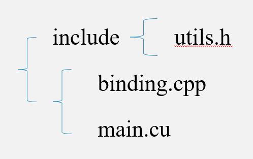
其中binding.cpp将建立cuda函数与python函数的接口，接下来我们将整个项目打包为python的一个package，名为PackBit：

setup.py

import glob
import os.path as osp
from setuptools import setup
from torch.utils.cpp_extension import CUDAExtension, BuildExtension

ROOT_DIR = osp.dirname(osp.abspath(__file__))
include_dirs = [osp.join(ROOT_DIR, "include")]

sources = glob.glob('*.cpp')+glob.glob('*.cu')


setup(
    name='PackBit',
    version='1.0',
    author='will'
    ext_modules=[
        CUDAExtension(
            name='PackBit',
            sources=sources,
            include_dirs=include_dirs,
            extra_compile_args={'cxx': ['-O2'],
                                'nvcc': ['-O2']}
        )
    ],
    cmdclass={
        'build_ext': BuildExtension
    }
)

由于我们跳过了CMakeLists.txt这一步，在编译cuda程序时不方便链接其他第三方库，这时我们可以在ext_modules添加参数library_dirs和libraries来额外指定所要链接的动态库，例如：

setup(
    name='PackBit',
    version='1.0',
    author='will',
    ext_modules=[
        CUDAExtension(
            name='PackBit',
            sources=sources,
            include_dirs=include_dirs,
            library_dirs=["/home/will/Downloads/libtorch/libtorch/lib","/usr/local/cuda-11.6/lib64"],
            libraries =["c10","torch_python","torch"],
            extra_compile_args={'cxx': ['-O2'],
                                'nvcc': ['-O2']},
            extra_link_args=["-Wl,-rpath=/home/will/Downloads/libtorch/libtorch/lib"]
        )
    ],
    cmdclass={#告诉编译器需要build
        'build_ext': BuildExtension
    }
)

将setup.py与main.cu和binding.cpp放在同一目录下，在bash中进入该目录，输入python setup.py install指令即可将该cuda程序编译并安装。

最后我们简单测试一下（需要注意，由于我们自己编写的studio库是基于torch库实现的，因此需要先import torch）：

test.py

import torch
import studio
import numpy as np
import math

if __name__ == "__main__":
    # 测试packbits
    a = torch.randint(2,(5463*3460,),dtype = torch.int32).cuda()
    b = torch.zeros([math.floor(5463*3460/32)],dtype = torch.int64).cuda()
    c=studio.packbits_u32(a,b)
    
    print('a前32位元素:',a[0:32])
    print('b[0]:',b[0])
    bin_str = "".format(b[0], 'b')
    print('b[0]的二进制形式：',np.binary_repr(b[0]).zfill(32))
    
    
    # 测试unpackbits
    # a = torch.zeros([5463*3460],dtype = torch.int32).cuda()
    # b = torch.randint(2**32,(math.floor(5463*3460/32),),dtype = torch.int64).cuda()
    # c=studio.un_packbits_u32(a,b)
    
    # print('b[0]:',b[0])
    # print('将b[0]解码后得到的向量',a[0:32])
    # bin_str = "".format(b[0], 'b')
    # print('b[0]的二进制形式：',np.binary_repr(b[0]).zfill(32))

测试结果：

packbits测试结果

unpackbits测试结果

3.3 debug

之前我们提到了cu算子with pybinding的方式不方便调试，想要调试只能另起一个C++项目，这里我们放上CMakeLists.txt文件以及main.cu

CMakeLists.txt

cmake_minimum_required(VERSION 2.8 FATAL_ERROR)
project(test)

find_package(PythonInterp REQUIRED)
find_package(CUDA REQUIRED)
# find_package(OpenCV)
find_package(Python3 COMPONENTS Interpreter Development REQUIRED)
find_package(Torch REQUIRED)

set(CMAKE_BUILD_TYPE DEBUG)
set(CMAKE_CUDA_COMPILER /usr/local/cuda-11.6/bin/nvcc)
set(CUDACXX /usr/local/cuda-11.6/bin/nvcc)
set(CMAKE_CXX_STANDARD 14)
set(Torch_DIR /home/will/Downloads/libtorch/libtorch/share/cmake/Torch)#使用torch库必须
set(CUDA_INCLUDE_DIRS "/usr/local/cuda/include")
include_directories(${PYTHON_INCLUDE_DIR})
include_directories(
        ./include
        /usr/include/python3.10
        # /usr/local/include/opencv4
        ${CUDA_INCLUDE_DIRS}
        )

set(LIBRARIES 
    # opencv_features2d
    # opencv_calib3d
    # opencv_flann
    # opencv_highgui
    # opencv_imgcodecs
    # opencv_imgproc
    # opencv_core
)

set(SRC_LIST ./main.cu)
add_executable(demo ${SRC_LIST})#将源文件变为可执行文件
target_link_libraries(demo "${TORCH_LIBRARIES}")#使用torch库必须
target_link_libraries(demo ${LIBRARIES})#将静态/动态库链接到可执行文件

main.cu

// #include "utils.h"
#include <torch/extension.h>
#include <iostream>
#include <ATen/ATen.h>
#include <ATen/TensorAccessor.h>
#include <ATen/cuda/CUDAContext.h>
#include <torch/extension.h>

using namespace std;

__global__ void packbits_u32_kernel(
    torch::PackedTensorAccessor32<int32_t,1,torch::RestrictPtrTraits> idx_array,
    torch::PackedTensorAccessor64<int64_t,1,torch::RestrictPtrTraits> bits_array
){
    // const int32_t n = blockIdx.x * blockDim.x + threadIdx.x;//一维时
    const int32_t n = blockIdx.x*blockDim.x*blockDim.y + threadIdx.x*blockDim.y + threadIdx.y;//二维时
    if(n > bits_array.size(0))
        return;
    int mask_size = 32;
    if (n == bits_array.size(0))
        mask_size = idx_array.size(0) % 32;
    const int64_t flag = 1;
    for(int i = 0 ; i < mask_size ; i++){
        int32_t hit_pix = idx_array[n*32 + i];
        // printf("asd");
        if (hit_pix > 0){
            bits_array[n] |= flag << i;
        }
    }
}


void packbits_u32_cu(
    torch::Tensor idx_array,
    torch::Tensor bits_array
){
    // 每个线程处理32位长数据即32个像素
    const int num_pixs = std::ceil(idx_array.size(0)/32);
    const int BLOCK_W = 64;
    const int BLOCK_H = 16;
    const dim3 blockSize(BLOCK_W,BLOCK_H,1);
    AT_DISPATCH_ALL_TYPES(idx_array.type(),"packbits_u64_cu",
    ([&] {
        packbits_u64_kernel<<<8, blockSize>>>(
            idx_array.packed_accessor32<int32_t,1,torch::RestrictPtrTraits>(),
            bits_array.packed_accessor64<int64_t,1,torch::RestrictPtrTraits>()
        );
    }));
}



int main() {
    auto data = torch::randint(0,2,{10000}).to(torch::kInt32);
    auto idx = torch::zeros({10}, torch::kInt64);

    auto data1 = data.to(torch::kCUDA);
    auto idx1 = idx.to(torch::kCUDA);

    packbits_u32_cu(data1,idx1);
    cudaDeviceSynchronize();
    auto modified_tensor = idx1.to(torch::kCPU);
    std::cout << idx1 << std::endl;

    return 0;
}

关于cuda的gdb调试我们不再介绍了，网上已有很多相关资料，可以参考cuda-gdb的官方文档

关于pybinding的c++配置，更详细的教程可以参考官方文档。

nerf_pl部分源码解读

nerf_pl是kwea123使用torchlightning复现的NeRF版本，相对于原版NeRF而言，代码易读易改，只是需要学习torchlightning，但我们可以结合gpt与官方api文档快速理解上手；接下来我们结合论文讲解一下nerf的网络结构和训练流程具体是怎样的。

该项目的主体在笔者看来主要包含三部分：模型、生成射线、渲染，项目的环境配置参考仓库的README即可。

1.模型部分

nerf的网络结构在models/nerf.py中：

class NeRF(nn.Module):
    def __init__(self,
                 D=8, W=256,
                 in_channels_xyz=63, in_channels_dir=27, 
                 skips=[4]):
        super(NeRF, self).__init__()
        self.D = D
        self.W = W
        self.in_channels_xyz = in_channels_xyz
        self.in_channels_dir = in_channels_dir
        self.skips = skips

        # xyz encoding layers
        for i in range(D):
            if i == 0:
                layer = nn.Linear(in_channels_xyz, W)
            elif i in skips:
                layer = nn.Linear(W+in_channels_xyz, W)
            else:
                layer = nn.Linear(W, W)
            layer = nn.Sequential(layer, nn.ReLU(True))
            setattr(self, f"xyz_encoding_{i+1}", layer)
        self.xyz_encoding_final = nn.Linear(W, W)

        # direction encoding layers
        self.dir_encoding = nn.Sequential(
                                nn.Linear(W+in_channels_dir, W//2),
                                nn.ReLU(True))

        # output layers
        self.sigma = nn.Linear(W, 1)
        self.rgb = nn.Sequential(
                        nn.Linear(W//2, 3),
                        nn.Sigmoid())

    def forward(self, x, sigma_only=False):
        if not sigma_only:
            input_xyz, input_dir = \
                torch.split(x, [self.in_channels_xyz, self.in_channels_dir], dim=-1)
        else:
            input_xyz = x

        xyz_ = input_xyz
        for i in range(self.D):
            if i in self.skips:
                xyz_ = torch.cat([input_xyz, xyz_], -1)
            xyz_ = getattr(self, f"xyz_encoding_{i+1}")(xyz_)

        sigma = self.sigma(xyz_)
        if sigma_only:
            return sigma

        xyz_encoding_final = self.xyz_encoding_final(xyz_)

        dir_encoding_input = torch.cat([xyz_encoding_final, input_dir], -1)
        dir_encoding = self.dir_encoding(dir_encoding_input)
        rgb = self.rgb(dir_encoding)

        out = torch.cat([rgb, sigma], -1)

        return out

我们可以看到整个网络其实很简单，NeRF类的网络结构包含一个 $8\times256$ 的MLP用于输出体密度与特征向量xyz_encoding_final，和一个一层MLP用于输出颜色，如下所示，其中embedding为：
$\gamma(p)=(sin(2^0\pi p),cos(2^0\pi p),...,sin(2^{L-1}\pi p),cos(2^{L-1}\pi p))$
nerf_pipeline

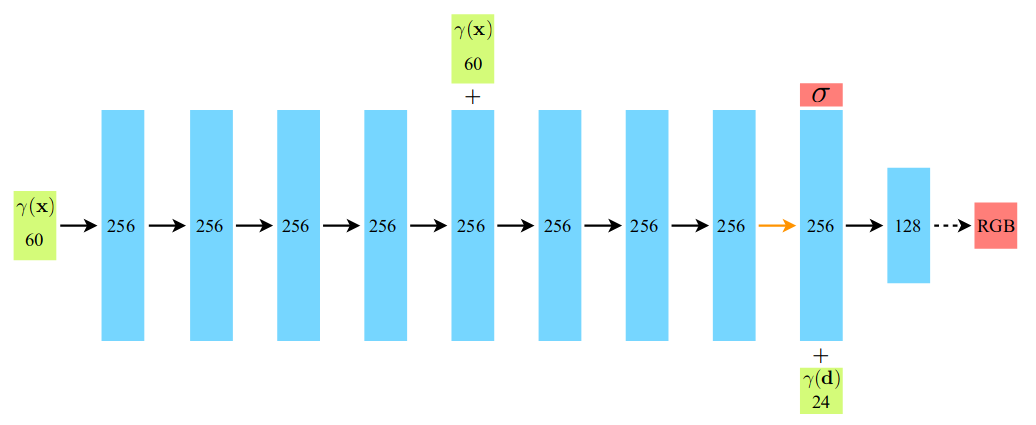
整个网络的输入是三维点数组x $\in R^{N\times3}$ 和观察到这些三维点的方向数组d $\in R^{N\times3}$ ；输出对应的rgb值rgb $\in R^{N\times3}$ 与体密度值sigma $\in R^{N}$

2.生成射线

生成射线的主体代码在datasets/ray_utils.py中，在get_rays函数中，输入参数directions表示在相机坐标系下，从相机光心到像素平面上个像素点的方向向量；c2w $= [R ∣ t]$ 表示由相机坐标系变换到世界坐标系下的变换矩阵：

def get_rays(directions, c2w):
    
    # Rotate ray directions from camera coordinate to the world coordinate
    rays_d = directions @ c2w[:, :3].T # (H, W, 3)
    rays_d = rays_d / torch.norm(rays_d, dim=-1, keepdim=True)
    # The origin of all rays is the camera origin in world coordinate
    rays_o = c2w[:, 3].expand(rays_d.shape) # (H, W, 3)

    rays_d = rays_d.view(-1, 3)
    rays_o = rays_o.view(-1, 3)

    return rays_o, rays_d

在该函数中，我们将相机坐标系下的方向向量directions通过c2w变换到世界坐标系下，就可以得到相机实际在真实空间下的视线：

direction

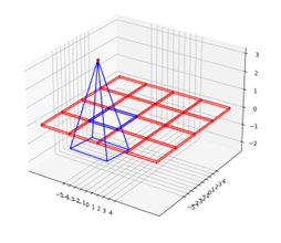
需要注意的是，该变换矩阵可以看作一个线性变换，在不同的基下，变换矩阵也是不同的，具体参照如下形式（其中BDF表示 $x, y, z$ 分别为右下前，BRU表示后右上）：

transform

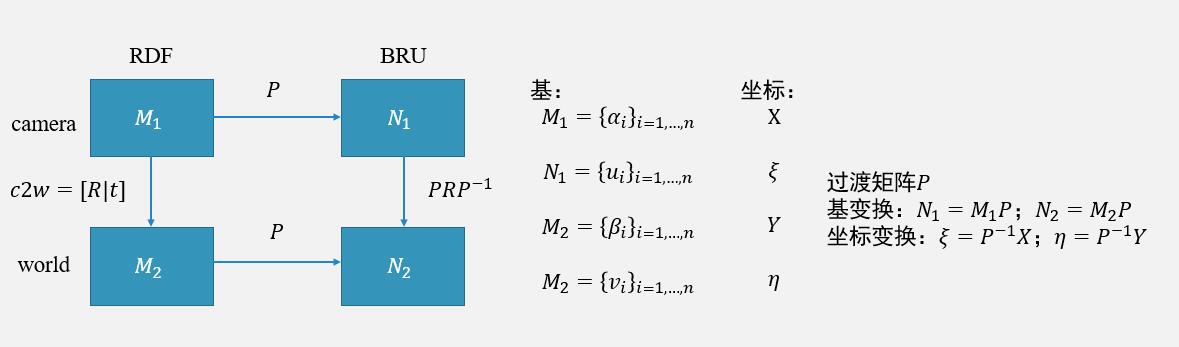
因此在llff以及blender数据集（这两个数据集的坐标系都是下右后）构造direction时：

directions = \
        torch.stack([(i-W/2)/focal, -(j-H/2)/focal, -torch.ones_like(i)], -1) # (H, W, 3)

而在使用colmap制作的数据集中，我们需要这样构造directions：

directions = \
        torch.stack([(u-cx+0.5)/fx, (v-cy+0.5)/fy, torch.ones_like(u)], -1)

当然我们也可以直接使用过渡矩阵对c2w进行相似变换，这与下图中的操作是等价的：

corrdinate

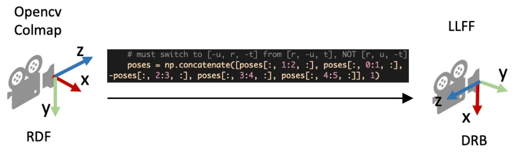
（上图来自博客）

总之，我们在使用c2w的时候，一定要先弄清楚c2w是哪个坐标系到哪个坐标系的变换。

3.渲染部分

nerf_pl渲染的主体在models/rendering.py中，这一部分比较复杂，但总体可以分为粗糙阶段采样，精细阶段采样。

其中inference函数代表一次前向过程，即，将(x,d)送入模型，输出对应的rgb与sigma，这个函数易于理解，对照我们在上一章中讲过的NeRF原理即可理解。nerf_pl将这个过程抽象出来有利于更简便地实现粗糙前向和精细前向：

粗糙前向：

		rgb_coarse, depth_coarse, weights_coarse = \
            inference(model_coarse, embedding_xyz, xyz_coarse_sampled, rays_d,
                      dir_embedded, z_vals, weights_only=False)
        result = {'rgb_coarse': rgb_coarse,
                  'depth_coarse': depth_coarse,
                  'opacity_coarse': weights_coarse.sum(1)
                 }

精细前向：

		rgb_fine, depth_fine, weights_fine = \
            inference(model_fine, embedding_xyz, xyz_fine_sampled, rays_d,
                      dir_embedded, z_vals, weights_only=False)

        result['rgb_fine'] = rgb_fine
        result['depth_fine'] = depth_fine
        result['opacity_fine'] = weights_fine.sum(1)

在粗糙前向结束后，我们会得到体渲染公式中的权重（在我们上一章中有详细介绍），通过sample_pdf

函数计算更准确的采样点位置，然后再将均匀采样点与精细采样点，一起送入精细前向进行体渲染。

4.训练过程

由于作者采用了torchlightning框架，大部分初学者在阅读其train.py时会比较懵，我们先给出一个pytorch_lightning.LightningModule在fit时，各个成员函数的执行顺序：

prepare_data()：该函数用于在开始训练之前加载数据集。它只会在单个进程中调用一次，通常在初始化训练模型之前调用。

setup()：该函数用于初始化模型和数据集。它在 prepare_data() 函数之后被调用，并在训练过程之前被调用。

train_dataloader()：该函数返回训练数据的数据加载器，它在 setup() 函数之后被调用。

val_dataloader()：该函数返回验证数据的数据加载器，它在 train_dataloader() 函数之后被调用。

test_dataloader()：该函数返回测试数据的数据加载器，它在 val_dataloader() 函数之后被调用。

forward()：该函数用于定义模型的前向传递过程，在训练和推理过程中被调用。

training_step()：该函数在每个训练批次（batch）中被调用，用于计算损失并执行反向传播。

validation_step()：该函数在每个验证批次（batch）中被调用，用于评估模型在验证集上的性能。

test_step()：该函数在每个测试批次（batch）中被调用，用于评估模型在测试集上的性能。

training_epoch_end()：该函数在每个训练轮次（epoch）结束时被调用，用于处理和汇总训练过程中的统计信息。

validation_epoch_end()：该函数在每个验证轮次（epoch）结束时被调用，用于处理和汇总验证过程中的统计信息。

test_epoch_end()：该函数在每个测试轮次（epoch）结束时被调用，用于处理和汇总测试过程中的统计信息。

configure_optimizers()：该函数用于定义优化器及其超参数，在训练过程之前被调用。

了解了这些成员方法的作用，则我们可以在初读时仅关注forward与training_step：

def training_step(self, batch, batch_nb):
        log = {'lr': get_learning_rate(self.optimizer)}
        rays, rgbs = self.decode_batch(batch)
        results = self(rays)
        log['train/loss'] = loss = self.loss(results, rgbs)
        typ = 'fine' if 'rgb_fine' in results else 'coarse'

        with torch.no_grad():
            psnr_ = psnr(results[f'rgb_{typ}'], rgbs)
            log['train/psnr'] = psnr_

        return {'loss': loss,
                'progress_bar': {'train_psnr': psnr_},
                'log': log
               }

torchlightning在加载完各个数据的dataloader后，会直接进入training_step，同时会传入data_loader中dataset的__getitem__()返回的数据，例如在datasets/blender.py中：

def __getitem__(self, idx):
        if self.split == 'train': # use data in the buffers
            sample = {'rays': self.all_rays[idx],
                      'rgbs': self.all_rgbs[idx]}

        else: # create data for each image separately
            frame = self.meta['frames'][idx]
            c2w = torch.FloatTensor(frame['transform_matrix'])[:3, :4]

            img = Image.open(os.path.join(self.root_dir, f"{frame['file_path']}.png"))
            img = img.resize(self.img_wh, Image.LANCZOS)
            img = self.transform(img) # (4, H, W)
            valid_mask = (img[-1]>0).flatten() # (H*W) valid color area
            img = img.view(4, -1).permute(1, 0) # (H*W, 4) RGBA
            img = img[:, :3]*img[:, -1:] + (1-img[:, -1:]) # blend A to RGB

            rays_o, rays_d = get_rays(self.directions, c2w)

            rays = torch.cat([rays_o, rays_d, 
                              self.near*torch.ones_like(rays_o[:, :1]),
                              self.far*torch.ones_like(rays_o[:, :1])],
                              1) # (H*W, 8)

            sample = {'rays': rays,
                      'rgbs': img,
                      'c2w': c2w,
                      'valid_mask': valid_mask}

        return sample

则在training_step中的输入参数batch即为上述的sample，然后training_step通过

results = self(rays)执行forward，并将前向得到的结果与原始图像rgbs作loss，loss在training_step之后会自动反传，不需要我们进行loss.backward与opt.step()

def forward(self, rays):
        """Do batched inference on rays using chunk."""
        B = rays.shape[0]
        results = defaultdict(list)
        for i in range(0, B, self.hparams.chunk):
            rendered_ray_chunks = \
                render_rays(self.models,
                            self.embeddings,
                            rays[i:i+self.hparams.chunk],
                            self.hparams.N_samples,
                            self.hparams.use_disp,
                            self.hparams.perturb,
                            self.hparams.noise_std,
                            self.hparams.N_importance,
                            self.hparams.chunk, # chunk size is effective in val mode
                            self.train_dataset.white_back)

            for k, v in rendered_ray_chunks.items():
                results[k] += [v]

        for k, v in results.items():
            results[k] = torch.cat(v, 0)
        return results