来源:《斯坦福数据挖掘教程·第三版》对应的公开英文书和PPT
Chapter 9 Recommendation SystemsRecommendation systems use a number of different technologies. We can classify these systems into two broad groups.
- Content-based systems examine properties of the items recommended. For instance, if a Netflix user has watched many cowboy movies, then recommend a movie classified in the database as having the “cowboy” genre.
- Collaborative filtering systems recommend items based on similarity measures between users and/or items. The items recommended to a user are those preferred by similar users. This sort of recommendation system can use the groundwork laid in Chapter 3 on similarity search and Chapter 7 on clustering. However, these technologies by themselves are not sufficient, and there are some new algorithms that have proven effective for recommendation systems.
In a recommendation-system application there are two classes of entities, which we shall refer to as users and items. Users have preferences for certain items, and these preferences must be teased out of the data. The data itself is represented as a utility matrix, giving for each user-item pair, a value that represents what is known about the degree of preference of that user for that item. Values come from an ordered set, e.g., integers 1–5 representing the number of stars
that the user gave as a rating for that item. We assume that the matrix is sparse, meaning that most entries are “unknown.” An unknown rating implies that we have no explicit information about the user’s preference for the item.
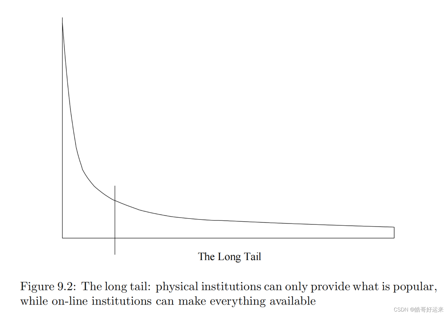
The distinction between the physical and on-line worlds has been called the long tail phenomenon, and it is suggested in Fig. 9.2. The vertical axis represents popularity (the number of times an item is chosen). The items are ordered on the horizontal axis according to their popularity. Physical institutions provide only the most popular items to the left of the vertical line, while the corresponding on-line institutions provide the entire range of items: the tail as well as the popular items.
Without a utility matrix, it is almost impossible to recommend items. However, acquiring data from which to build a utility matrix is often difficult. There are two general approaches to discovering the value users place on items.
- We can ask users to rate items. Movie ratings are generally obtained this way, and some on-line stores try to obtain ratings from their purchasers. Sites providing content, such as some news sites or YouTube also ask users to rate items. This approach is limited in its effectiveness, since generally users are unwilling to provide responses, and the information from those who do may be biased by the very fact that it comes from people willing to provide ratings.
- We can make inferences from users’ behavior. Most obviously, if a user buys a product at Amazon, watches a movie on YouTube, or reads a news article, then the user can be said to “like” this item. Note that this sort of rating system really has only one value: 1 means that the user likes the item. Often, we find a utility matrix with this kind of data shown with 0’s rather than blanks where the user has not purchased or viewed the item. However, in this case 0 is not a lower rating than 1; it is no rating at all. More generally, one can infer interest from behavior other than purchasing. For example, if an Amazon customer views information about an item, we can infer that they are interested in the item, even if they don’t buy it.
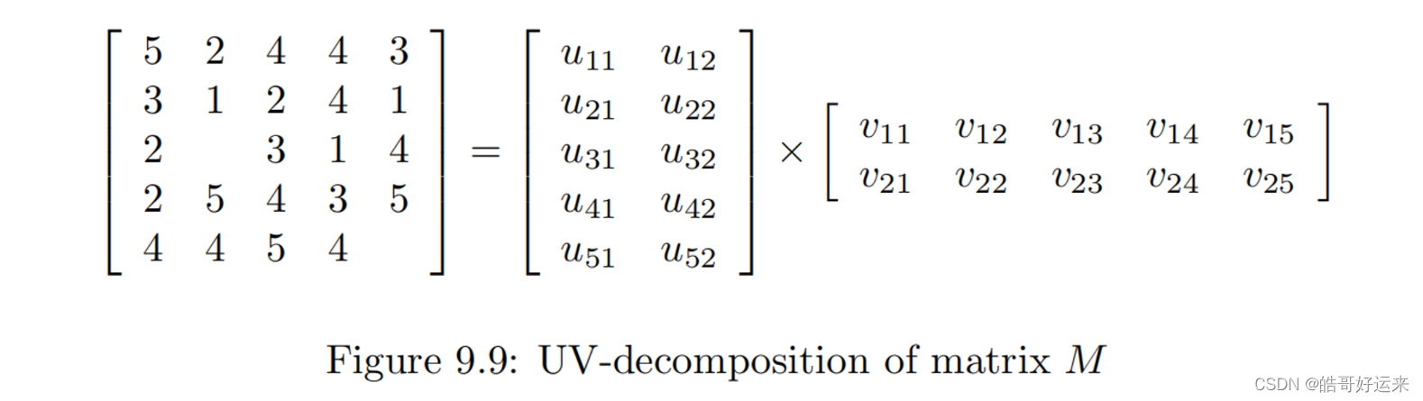
Consider movies as a case in point. Most users respond to a small number of features; they like certain genres, they may have certain famous actors or actresses that they like, and perhaps there are a few directors with a significant following. If we start with the utility matrix M, with n rows and m columns (i.e., there are n users and m items), then we might be able to find a matrix
U with n rows and d columns and a matrix V with d rows and m columns, such that UV closely approximates M in those entries where M is nonblank. If so, then we have established that there are d dimensions that allow us to characterize both users and items closely. We can then use the entry in the product UV to estimate the corresponding blank entry in utility matrix M. This process is called UV-decomposition of M.
While we can pick among several measures of how close the product UV is to M, the typical choice is the root-mean-square error (RMSE), where we
- Sum, over all nonblank entries in M the square of the difference between that entry and the corresponding entry in the product UV .
- Take the mean (average) of these squares by dividing by the number of terms in the sum (i.e., the number of nonblank entries in M).
- Take the square root of the mean.
Building a Complete UV-Decomposition Algorithm
Preprocessing
Because the differences in the quality of items and the rating scales of users are such important factors in determining the missing elements of the matrix M, it is often useful to remove these influences before doing anything else.
We can subtract from each nonblank element
m
i
j
m_{ij}
mij the average rating of user i. Then, the resulting matrix can be modified by subtracting the average rating (in the modified matrix) of item j. It is also possible to first subtract the average rating of item j and then subtract the
average rating of user i in the modified matrix. The results one obtains from doing things in these two different orders need not be the same, but will tend to be close. A third option is to normalize by subtracting from
m
i
j
m_{ij}
mij the average of the average rating of user i and item j, that is, subtracting one half the sum of the user average and the item average. If we choose to normalize M, then when we make predictions, we need to undo the normalization. That is, if whatever prediction method we use results in estimate e for an element
m
i
j
m_{ij}
mij of the normalized matrix, then the value we predict for
m
i
j
m_{ij}
mij in the true utility matrix is e plus whatever amount was subtracted from row i and from column j during the normalization process.
Initialization
As we mentioned, it is essential that there be some randomness in the way we seek an optimum solution, because the existence of many local minima justifies our running many different optimizations in the hope of reaching the global minimum on at least one run. We can vary the initial values of U and V , or we can vary the way we seek the optimum (to be discussed next), or both. A simple starting point for U and V is to give each element the same value, and a good choice for this value is that which gives the elements of the product UV the average of the nonblank elements of M. Note that if we have normalized M, then this value will necessarily be 0. If we have chosen d as the lengths of the short sides of U and V , and a is the average nonblank element of M, then the elements of U and V should be
a
/
d
\sqrt {a/d}
a/d.
If we want many starting points for U and V , then we can perturb the value
a
/
d
\sqrt {a/d}
a/d randomly and independently for each of the elements. There are many options for how we do the perturbation. We have a choice regarding the distribution of the difference. For example we could add to each element a normally distributed value with mean 0 and some chosen standard deviation. Or we could add a value uniformly chosen from the range
−
c
−c
−c to
+
c
+c
+c for some c.
Performing the Optimization
In order to reach a local minimum from a given starting value of U and V , we need to pick an order in which we visit the elements of U and V . The simplest thing to do is pick an order, e.g., row-by-row, for the elements of U and V , and visit them in round-robin fashion. Note that just because we optimized an element once does not mean we cannot find a better value for that element after other elements have been adjusted. Thus, we need to visit elements repeatedly, until we have reason to believe that no further improvements are possible.
Alternatively, we can follow many different optimization paths from a single starting value by randomly picking the element to optimize. To make sure that every element is considered in each round, we could instead choose a permutation of the elements and follow that order for every round.
Converging to a Minimum
Ideally, at some point the RMSE becomes 0, and we know we cannot do better. In practice, since there are normally many more nonblank elements in M than there are elements in U and V together, we have no right to expect that we can reduce the RMSE to 0. Thus, we have to detect when there is little benefit to be had in revisiting elements of U and/or V . We can track the amount of improvement in the RMSE obtained in one round of the optimization, and stop when that improvement falls below a threshold. A small variation is to observe the improvements resulting from the optimization of individual elements, and stop when the maximum improvement during a round is below a threshold.
Avoiding Overfitting
One problem that often arises when performing a UV-decomposition is that we arrive at one of the many local minima that conform well to the given data, but picks up values in the data that don’t reflect well the underlying process that gives rise to the data. That is, although the RMSE may be small on the given data, it doesn’t do well predicting future data. There are several things that can be done to cope with this problem, which is called overfitting by statisticians.
- Avoid favoring the first components to be optimized by only moving the value of a component a fraction of the way, say half way, from its current value toward its optimized value.
- Stop revisiting elements of U and V well before the process has converged.
- Take several different UV decompositions, and when predicting a new entry in the matrix M, take the average of the results of using each decomposition.
Summary of Chapter 9
- Utility Matrices: Recommendation systems deal with users and items. A utility matrix offers known information about the degree to which a user likes an item. Normally, most entries are unknown, and the essential problem of recommending items to users is predicting the values of the unknown entries based on the values of the known entries.
- Two Classes of Recommendation Systems: These systems attempt to predict a user’s response to an item by discovering similar items and the response of the user to those. One class of recommendation system is content-based; it measures similarity by looking for common features of the items. A second class of recommendation system uses collaborative filtering; these measure similarity of users by their item preferences and/or measure similarity of items by the users who like them.
- Item Profiles: These consist of features of items. Different kinds of items have different features on which content-based similarity can be based. Features of documents are typically important or unusual words. Products have attributes such as screen size for a television. Media such as movies have a genre and details such as actor or performer. Tags can also be used as features if they can be acquired from interested users.
- User Profiles: A content-based collaborative filtering system can construct profiles for users by measuring the frequency with which features appear in the items the user likes. We can then estimate the degree to which a user will like an item by the closeness of the item’s profile to the user’s profile.
- Classification of Items: An alternative to constructing a user profile is to build a classifier for each user, e.g., a decision tree. The row of the utility matrix for that user becomes the training data, and the classifier must predict the response of the user to all items, whether or not the row had an entry for that item.
- Similarity of Rows and Columns of the Utility Matrix : Collaborative filtering algorithms must measure the similarity of rows and/or columns of the utility matrix. Jaccard distance is appropriate when the matrix consists only of 1’s and blanks (for “not rated”). Cosine distance works for more general values in the utility matrix. It is often useful to normalize the utility matrix by subtracting the average value (either by row, by column, or both) before measuring the cosine distance.
- Clustering Users and Items: Since the utility matrix tends to be mostly blanks, distance measures such as Jaccard or cosine often have too little data with which to compare two rows or two columns. A preliminary step or steps, in which similarity is used to cluster users and/or items into small groups with strong similarity, can help provide more common components with which to compare rows or columns.
- UV-Decomposition: One way of predicting the blank values in a utility matrix is to find two long, thin matrices U and V , whose product is an approximation to the given utility matrix. Since the matrix product UV gives values for all user-item pairs, that value can be used to predict the value of a blank in the utility matrix. The intuitive reason this method makes sense is that often there are a relatively small number of issues (that
number is the “thin” dimension of U and V ) that determine whether or not a user likes an item. - Root-Mean-Square Error : A good measure of how close the product UV is to the given utility matrix is the RMSE (root-mean-square error). The RMSE is computed by averaging the square of the differences between UV and the utility matrix, in those elements where the utility matrix is nonblank. The square root of this average is the RMSE.
- Computing U and V : One way of finding a good choice for U and V in a UV decomposition is to start with arbitrary matrices U and V . Repeatedly adjust one of the elements of U or V to minimize the RMSE between the product UV and the given utility matrix. The process converges to a local optimum, although to have a good chance of obtaining a global optimum we must either repeat the process from many starting matrices, or search from the starting point in many different ways.
END


![【群智能算法改进】一种改进的沙丘猫群优化算法 改进沙丘猫群算法 改进SCSO[1]【Matlab代码#34】](https://img-blog.csdnimg.cn/e95879a529e04ce796e80c5913678e4d.png#pic_center)