<~生~信~交~流~与~合~作~请~关~注~公~众~号@生信探索>

中心极限定律

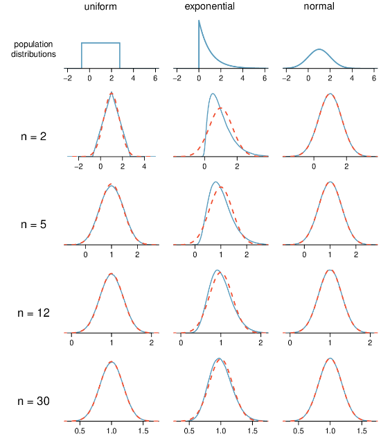
中心极限定律：当样本样足够大时（n≥30），样本的mean等于总体的mean

例如，对学校的学生身高抽样，100组每组30人，每组的身高均值分别为 ，那么可以画出 的频数图，应该是正态分布的。

一般性结论，即使整体服从不同的分布他们的means也服从正态分布。

For samples of size 30 or more, the sample mean is approximately normally distributed

正态分布

正态分布（Normal distribution），也称“常态分布”，又名高斯分布（Gaussian distribution）。若随机变量X服从一个数学期望为μ、方差为σ2的正态分布，记为N(μ，σ2)。其概率密度函数为正态分布的期望值μ决定了其位置，其标准差σ决定了分布的幅度。当μ = 0,σ = 1时的正态分布是标准正态分布。

Z分布，即标准正态分布，z=(x−μ)/σ，Z值可以查表。

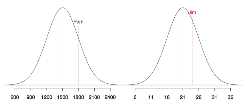
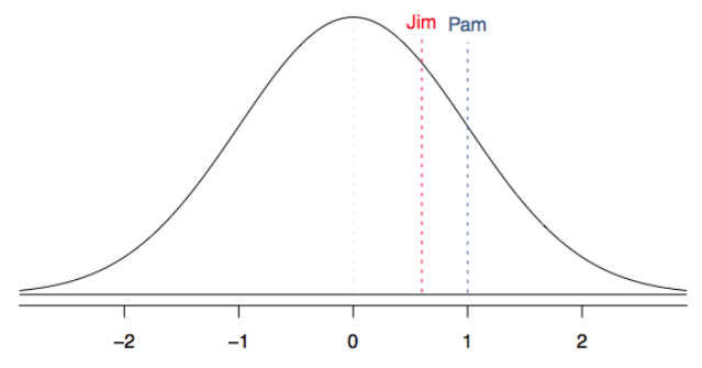
例题：SAT scores are distributed nearly normally with mean 1500 and standard deviation 300. ACT scores are distributed nearly normally with mean 21 and standard deviation 5. A college admissions officer wants to determine which of the two applicants scored better on their standardized test with respect to the other test takers: Pam, who earned an 1800 on her SAT, or Jim, who scored a 24 on his ACT?

解：

Standardizing with Z scores

Since we cannot just compare these two raw scores, we instead compare how many standard deviations beyond the mean each observation is.

• Pam's score is (1800 - 1500) / 300 = 1 standard deviation above the mean.
• Jim's score is (24 - 21) / 5 = 0.6 standard deviations above the mean.

So Pam is better.

z-score

z-scores are the signed number of standard deviations above the mean that an observation lies, z=(x−μ)/σ

即把数据转换为z分布(标准正态分布)。

• python

axis=0时对列z-score处理

ddof=1的意思是（自由度）计算标准差中分母上是n-1，默认是n-0，n就是样本数；当axis=0时，n=5

import numpy as np
from scipy.stats import zscore
m = np.array([[ 0.3148,  0.0478,  0.6243,  0.4608],
              [ 0.7149,  0.0775,  0.6072,  0.9656],
              [ 0.6341,  0.1403,  0.9759,  0.4064],
              [ 0.5918,  0.6948,  0.904 ,  0.3721],
              [ 0.0921,  0.2481,  0.1188,  0.1366]])

zscore(m, axis=1, ddof=0)

• julia

默认对行z-score处理，std计算时默认的分母是n-1，默认对行zscore处理，所以对m转制

using StatsBase
m = [0.3148  0.0478 0.6243 0.4608
  0.7149 0.0775 0.6072 0.9656
  0.6341 0.1403 0.9759 0.4064
  0.5918 0.6948 0.904 0.3721
  0.0921 0.2481 0.1188 0.1366]
μ = mean.(eachrow(m'))
σ = std.(eachrow(m'))
z=zscore(m', μ, σ)
z'

• R

默认对列z-score处理，std计算时默认的分母是n-1

m = matrix(c(0.3148,  0.0478,  0.6243,  0.4608,
  0.7149,  0.0775,  0.6072,  0.9656,
  0.6341,  0.1403,  0.9759,  0.4064,
  0.5918,  0.6948,  0.904 ,  0.3721,
  0.0921,  0.2481,  0.1188,  0.1366)
  ,ncol=4,byrow=T)
scale(m)

Reference

https://spot.pcc.edu/math/ahss/ed2/distributionofxbar.html
https://www.bilibili.com/video/BV1CA411P7bL
https://stats.libretexts.org/Bookshelves/Introductory_Statistics/Introductory_Statistics_(Shafer_and_Zhang)/06%3A_Sampling_Distributions/6.02%3A_The_Sampling_Distribution_of_the_Sample_Mean
https://zhuanlan.zhihu.com/p/141732064
https://baike.baidu.com/item/Z%E5%88%86%E6%95%B0/8268473
https://people.umass.edu/biep540w/pdf/Open%20Intro%20Slides%20-%20Normal%20Distribution.pdf#:~:text=SAT%20scores%20are%20distributed%20nearly%20normally%20with%20mean,Jim%2C%20who%20scored%20a%2024%20on%20his%20ACT%3F