间歇采样直接、重复、循环转发干扰
间歇采样转发干扰是在雷达脉冲周期内对雷达信号进行间歇采样,并通过干扰机将采样的信号进行处理和转发,从而生成相干的假目标信号。这种干扰方式的原理可分为直接转发、重复转发和逐次循环转发三种方式。直接转发是指在两段采样操作之间,干扰机对已采样信号进行直接转发;重复转发是当干扰机截获到一段雷达信号后,对其进行采样生成采样信号,根据设定的重复次数,对该采样信号进行重复转发;逐次循环转发则是按照预先设定的顺序依次对采样信号进行处理和转发。
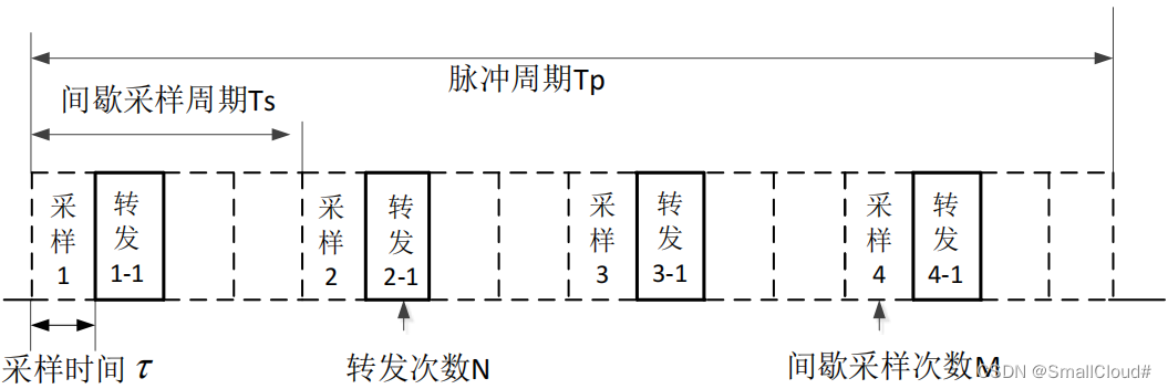
间歇采样信号模型如图下图所示,其脉冲持续时间为 τ \tau τ ,重复周期为 T s T_s Ts ,矩形包络脉冲为:
p ( t ) = rect ( t τ ) ∗ ∑ − ∞ ∞ δ ( t − n T s ) p(t)=\operatorname{rect}\left(\frac{t}{\tau}\right) * \sum_{-\infty}^{\infty} \delta\left(t-n T_s\right) p(t)=rect(τt)∗−∞∑∞δ(t−nTs)

利用傅里叶变换关系:
rect
(
t
τ
)
↔
τ
S
a
(
π
f
τ
)
,
∑
−
∞
∞
δ
(
t
−
n
T
s
)
↔
1
T
s
∑
−
∞
∞
δ
∣
f
−
f
s
∣
\operatorname{rect}\left(\frac{t}{\tau}\right) \leftrightarrow \tau S a(\pi f \tau), \quad \sum_{-\infty}^{\infty} \delta\left(t-n T_s\right) \leftrightarrow \frac{1}{T_s} \sum_{-\infty}^{\infty} \delta\left|f-f_s\right|
rect(τt)↔τSa(πfτ),−∞∑∞δ(t−nTs)↔Ts1−∞∑∞δ∣f−fs∣
其中
f
s
=
1
T
s
\displaystyle{f_s=\frac{1}{T_s}}
fs=Ts1 为采样频率,
S
a
(
x
)
=
sin
(
x
)
/
x
S a(x)=\sin (x) / x
Sa(x)=sin(x)/x ,
p
(
t
)
p(t)
p(t) 的频谱为:
P ( f ) = ∑ − ∞ ∞ τ f s S a ( π n f s τ ) δ ( f − n f s ) = ∑ − ∞ ∞ a n δ ( f − n f s ) P(f)=\sum_{-\infty}^{\infty} \tau f_s S a\left(\pi n f_s \tau\right) \delta\left(f-n f_s\right)=\sum_{-\infty}^{\infty} a_n \delta\left(f-n f_s\right) P(f)=−∞∑∞τfsSa(πnfsτ)δ(f−nfs)=−∞∑∞anδ(f−nfs)
其中 a n = τ f s S a ( π n f s τ ) a_n=\tau f_s S a\left(\pi n f_s \tau\right) an=τfsSa(πnfsτ). 特别的, 当 T s = 2 τ T_s=2 \tau Ts=2τ 时, p ( t ) p(t) p(t) 变成方波脉冲串,上式变成
P ( f ) = ∑ − ∞ + ∞ 1 2 S a ( n π 2 ) δ ( f − n f s ) P(f)=\sum_{-\infty}^{+\infty} \frac{1}{2} S a\left(\frac{n \pi}{2}\right) \delta\left(f-n f_s\right) P(f)=−∞∑+∞21Sa(2nπ)δ(f−nfs)
设雷达发射信号
x
(
t
)
x(t)
x(t) 的频谱为
X
(
f
)
X(f)
X(f) 。干扰机对雷达信号采样得到采样信号为:
x
s
(
t
)
=
p
(
t
)
x
(
t
)
x_s(t)=p(t) x(t)
xs(t)=p(t)x(t)
频谱为:
X
s
(
f
)
=
P
(
f
)
∗
X
(
f
)
=
∑
−
∞
∞
a
n
X
(
f
−
n
f
s
)
X_s(f)=P(f) * X(f)=\sum_{-\infty}^{\infty} a_n X\left(f-n f_s\right)
Xs(f)=P(f)∗X(f)=−∞∑∞anX(f−nfs)
可以看出
X
s
(
f
)
X_s(f)
Xs(f) 是
X
(
f
)
X(f)
X(f) 的周期加权延拓, 延拓周期为
T
s
T_s
Ts, 幅度加权系数为
a
n
a_n
an, 根根据信号与系统知识可知,间歇采样干扰将产生一个主假目标以及一系列在主假目标旁逐渐衰减的次假目标。
间歇采样直接转发干扰仅需测量出雷达信号的脉宽即可开展干扰,图\ref{间歇采样直接转发干扰原理示意图}给出了间歇采样直接转发干扰的原理模型。
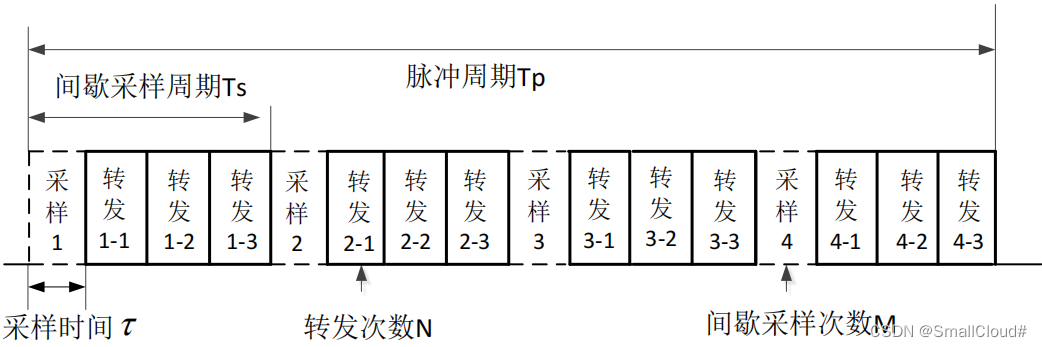
图\ref{间歇采样重复转发干扰原理示意图}给出了间歇采样重复转发干扰最简单的一种形式,可以看出,如果转发次数只有一次,那么此时就等效于占空比为50 %的间歇采样直接转发干扰,转发1-2、2-2、3-2、4-2可以认为是第一次转发信号延时 τ \tau τ 后的转发干扰,设第一次转发干扰信号为 y s ( t ) \displaystyle{y_{s}(t)} ys(t) ,则第二次转发输出信号为 y s ( t − τ ) \displaystyle{y_{s}(t-\tau)} ys(t−τ) ;每多重复转发一次,输出信号需在前一次输出信号的基础上延时 τ \tau τ ,直至完成最后一次转发,即 y s ( t ) \displaystyle{y_{s}(t)} ys(t) 以 τ \tau τ 为间隔延拓了 M s M_s Ms 次,容易得出 M s = T s / τ − 1 M_s={T_s}/{\tau}-1 Ms=Ts/τ−1 ,则总的干扰输出信号可以表示为:
y s ( t ) + y s ( t − τ ) + ⋯ + y s ( t − ( M s − 1 ) τ ) = ∑ r = 0 M s − 1 y s ( t − r τ ) y_s(t)+y_s(t-\tau)+\cdots+y_s\left(t-\left(M_s-1\right) \tau\right)=\sum_{r=0}^{M_s-1} y_s(t-r \tau) ys(t)+ys(t−τ)+⋯+ys(t−(Ms−1)τ)=r=0∑Ms−1ys(t−rτ)
间歇采样转发干扰能够较好地适应各种雷达信号处理系统,并且不易被探测和干扰,因此在现代雷达干扰中使用较为广泛,但目前的间歇采样转发干扰技术多是以采样不连续的情况下进行的,干扰回波与真实回波存在差别,可以结合其他干扰技术以提高干扰效果。
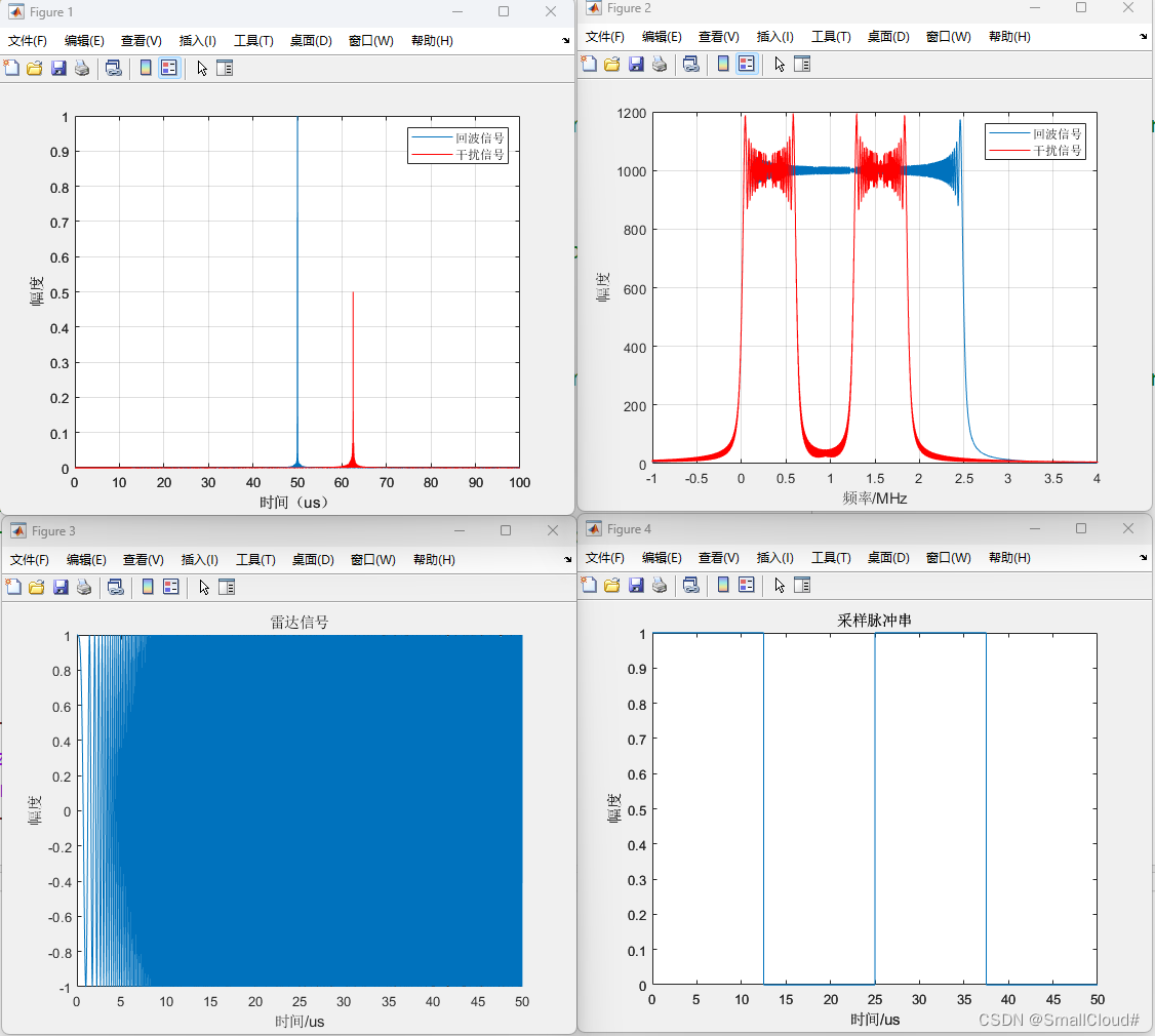
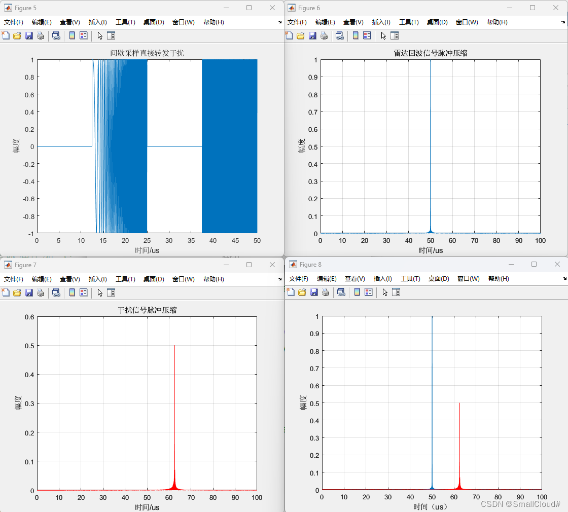
1、间歇采样直接转发干扰-仿真
clc;clear;close all
% 间歇采样直接转发干扰 20230505
Tp = 50e-6; %雷达信号脉宽50us
B = 50e6; %雷达信号带宽50MHz
mu = B/Tp; %调频斜率
%Ts_jam =10e-6;
%Ts_jam =20e-6; %间歇采样干扰的采样周期
%Ts_jam =0.1e-6;
Ts_jam =25e-6;
%tao_jam = 5e-6; %间歇采样干扰的采样脉宽5us
tao_jam = 12.5e-6;
fs = 20*B;
Ts = 1/fs;
T_sample =Tp; %采样时间
N_sample = ceil(T_sample/Ts);
N_sample_tao_jam = ceil(tao_jam/Ts);
N_sample_Ts_jam = ceil(Ts_jam/Ts);
%% 坐标轴变量
t = linspace(0,T_sample,N_sample);
%% 回波信号
Sig_rec = exp(1i*pi*mu*(t).^2);
%% 间歇采样干扰
%% 采样脉冲
Sig_pulse = zeros(1,N_sample);
N_jam = Tp/Ts_jam; %干扰采样次数,即采样脉冲个数
for ii = 1:N_jam
Sig_pulse( (1+ (ii-1)*N_sample_Ts_jam) :N_sample_tao_jam + (ii-1)*N_sample_Ts_jam) = 1;
end
%% 干扰信号
Sig_jam = Sig_rec.*Sig_pulse;
Sig_jam = [Sig_jam(N_sample-N_sample_tao_jam+1:N_sample),Sig_jam(1:N_sample-N_sample_tao_jam)];
%% 脉冲压缩
N_fft = 2*N_sample; % fft点数
%% 参考信号
Sig_ref = exp(1i*pi*mu*(t).^2);
F_Sig_ref = fft(Sig_ref,N_fft);
%% 雷达信号的脉冲压缩
PC_Sig_rec = fftshift( ifft(fft(Sig_rec,N_fft).*(conj(F_Sig_ref))) );
%1 PC_Sig_rec = PC_Sig_rec(1:N_sample);
%% 干扰信号的脉冲压缩
PC_Sig_jam = fftshift( ifft(fft(Sig_jam,N_fft).*(conj(F_Sig_ref))) );
%2 PC_Sig_jam = PC_Sig_jam(1:N_sample);
%% 画图
testpara_t = linspace(0,2*Tp,2*N_sample);
para_norm = max( abs( real( PC_Sig_rec ) ) );
figure;
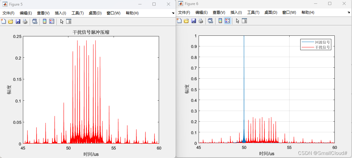
plot(testpara_t*1e6,( abs( real( PC_Sig_rec ) )/para_norm ));
%plot(testpara_t*1e6,( abs( real( PC_Sig_rec ) )/para_norm )/max(( abs( real( PC_Sig_rec ) )/para_norm )));
xlabel('时间/us');ylabel('幅度');
%title('雷达回波信号脉冲压缩');
%xlim([96 104]);
%plot(testpara_t*1e6,20*log10( abs( real( PC_Sig_rec ) )/para_norm ));
grid on;
hold on;
plot(testpara_t*1e6,( abs( real( PC_Sig_jam ) )/para_norm ),'r');
%plot(testpara_t*1e6,( abs( real( PC_Sig_jam ) )/para_norm )/max(( abs( real( PC_Sig_jam ) )/para_norm )));
xlabel('时间(us)');ylabel('幅度');
%title('干扰信号脉冲压缩');
%xlim([48 65]);% 占空比0.5
%xlim([48 57]);% 占空比0.2
%plot(testpara_t*1e6,20*log10( abs( real( PC_Sig_jam ) )/para_norm ));
grid on;legend('回波信号','干扰信号');
% figure%画出来的不对
% N = fs*Tp;
% freq = linspace(-B/2, B/2, N);
% plot(freq/1e6, fftshift(abs(fft(Sig_rec))));
% xlabel('频率/MHz');ylabel('幅度');
% grid on; hold on;
% plot(freq/1e6, fftshift(abs(fft(Sig_jam))),'r');
% xlim([-1 4]);
% legend('回波信号','干扰信号');
figure;
plot(t*1e6,real(Sig_rec));
xlabel('时间/us');ylabel('幅度');
title('雷达信号');
figure;
plot(t*1e6,Sig_pulse);
xlabel('时间/us');ylabel('幅度');
title('采样脉冲串');
figure;
plot(t*1e6,real(Sig_jam));
xlabel('时间/us');ylabel('幅度');
title('间歇采样直接转发干扰');
testpara_t = linspace(0,2*Tp,2*N_sample);
para_norm = max( abs( real( PC_Sig_rec ) ) );
figure;
plot(testpara_t*1e6,( abs( real( PC_Sig_rec ) )/para_norm ));
xlabel('时间/us');ylabel('幅度');
title('雷达回波信号脉冲压缩');
%xlim([]);
%plot(testpara_t*1e6,20*log10( abs( real( PC_Sig_rec ) )/para_norm ));
grid on;
figure;
plot(testpara_t*1e6,( abs( real( PC_Sig_jam ) )/para_norm ),'r');
xlabel('时间/us');ylabel('幅度');
title('干扰信号脉冲压缩');
%xlim([]);
%plot(testpara_t*1e6,20*log10( abs( real( PC_Sig_jam ) )/para_norm ));
grid on;
figure;
plot(testpara_t*1e6,( abs( real( PC_Sig_rec ) )/para_norm ),'Linewidth',0.7);
xlabel('时间(us)');ylabel('幅度');
%xlim([95 110]);
hold on;
plot(testpara_t*1e6,( abs( real( PC_Sig_jam ) )/para_norm ),'r','Linewidth',0.7);
grid on;
需要注意,图二是不对的,代码中对其进行了注释
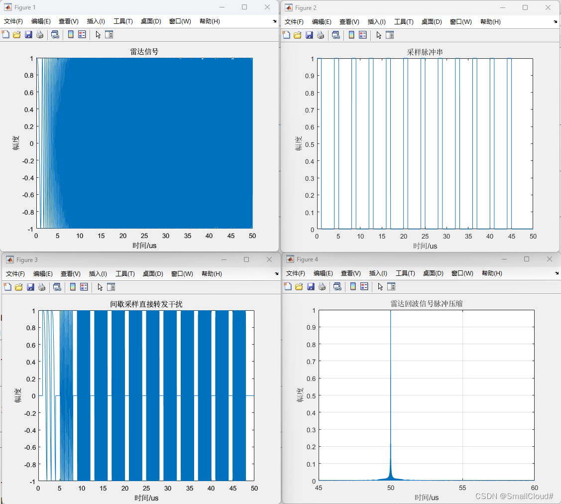
2、间歇采样重复转发干扰-仿真
clc;clear;close all
%间歇采样重复转发干扰--20230505
Tp = 50e-6;                 %雷达信号脉宽50us
B = 50e6;                   %雷达信号带宽50MHz
mu = B/Tp;                  %调频斜率
%%
% Ts_jam = 8e-6;              %间歇采样干扰的采样周期8us
% tao_jam = 1e-6;             %间歇采样干扰的采样脉宽1us
%%
Ts_jam = 4e-6;
tao_jam = 1e-6;
%%
M = round(Ts_jam/tao_jam -1);          % 延拓次数
fs = 10*B;
Ts = 1/fs;
T_sample =Tp;               %采样时间
N_sample = ceil(T_sample/Ts);
N_sample_tao_jam = ceil(tao_jam/Ts);
N_sample_Ts_jam = ceil(Ts_jam/Ts);
%% 坐标轴变量
t = linspace(0,T_sample,N_sample);

%% 回波信号
Sig_rec = exp(1i*pi*mu*(t).^2);

%% 间歇采样干扰
    %% 采样脉冲
    Sig_pulse = zeros(1,N_sample);
    N_jam = Tp/Ts_jam;      %干扰采样次数,即采样脉冲个数
    for ii = 1:N_jam
    Sig_pulse( (1+ (ii-1)*N_sample_Ts_jam) :N_sample_tao_jam + (ii-1)*N_sample_Ts_jam) = 1;
    end
    %% 干扰信号
    Sig_jam = Sig_rec.*Sig_pulse;
%     Sig_jam1 = [zeros(1,N_sample_tao_jam),Sig_jam];
%     Sig_jam2 = [zeros(1,N_sample_tao_jam),Sig_jam1];
%     Sig_jam3 = [zeros(1,N_sample_tao_jam),Sig_jam2];
    Sig_jam_matrix = zeros(M+1,(N_sample+(M)*N_sample_tao_jam));
    Sig_jam_matrix(1,1:length(Sig_jam)) = Sig_jam;
    for ii =2:M+1
        Sig_jam_matrix(ii,1:( length(Sig_jam)+(ii-1)*N_sample_tao_jam )) = [zeros(1,N_sample_tao_jam),Sig_jam_matrix(ii-1,1:(length(Sig_jam)+(ii-2)*N_sample_tao_jam))];
    end
    %% 归零
    Sig_jam = zeros(1,N_sample);
    for ii = 2:M+1
        Sig_jam = Sig_jam+Sig_jam_matrix(ii,1:N_sample);
    end

%% 脉冲压缩
    N_fft = 2*N_sample;         % fft点数
    %% 参考信号
    Sig_ref = exp(1i*pi*mu*(t).^2);
    F_Sig_ref = fft(Sig_ref,N_fft);
    %% 雷达信号的脉冲压缩
    PC_Sig_rec = fftshift( ifft(fft(Sig_rec,N_fft).*(conj(F_Sig_ref))) );
    %1 PC_Sig_rec = PC_Sig_rec(1:N_sample);
    %% 干扰信号的脉冲压缩
    PC_Sig_jam = fftshift( ifft(fft(Sig_jam,N_fft).*(conj(F_Sig_ref))) );
    %2 PC_Sig_jam = PC_Sig_jam(1:N_sample);
%% 画图
figure;
plot(t*1e6,real(Sig_rec));
xlabel('时间/us');ylabel('幅度');
title('雷达信号');

figure;
plot(t*1e6,Sig_pulse);
xlabel('时间/us');ylabel('幅度');
title('采样脉冲串');

t_jam = (1:length(Sig_jam))*Ts;
figure;
plot(t_jam*1e6,real(Sig_jam));
xlabel('时间/us');ylabel('幅度');
title('间歇采样直接转发干扰');

testpara_t = linspace(0,2*Tp,2*N_sample);
para_norm = max( abs( real( PC_Sig_rec ) ) );
figure;
plot(testpara_t*1e6,( abs( real( PC_Sig_rec ) )/para_norm ));
xlabel('时间/us');ylabel('幅度');xlim([45,60]);
title('雷达回波信号脉冲压缩');
%plot(testpara_t*1e6,20*log10( abs( real( PC_Sig_rec ) )/para_norm ));
grid on;

testpara_t_jam = (1:length(PC_Sig_jam))*Ts;
figure;
plot(testpara_t_jam*1e6,( abs( real( PC_Sig_jam ) )/para_norm ),'r');
xlabel('时间/us');ylabel('幅度');
title('干扰信号脉冲压缩');xlim([45,60]);
testpara_t = linspace(0,2*Tp,2*N_sample);
para_norm = max( abs( real( PC_Sig_rec ) ) );

figure;
plot(testpara_t*1e6,( abs( real( PC_Sig_rec ) )/para_norm )/max(( abs( real( PC_Sig_rec ) )/para_norm )));
xlabel('时间/us');ylabel('幅度');
hold on;
xlim([45,60]);
plot(testpara_t*1e6, (abs( real( PC_Sig_jam ) )/para_norm)/max(abs( real( PC_Sig_rec ) )/para_norm) ,'r');
grid on;
legend('回波信号','干扰信号');

% % 绘制频谱图
% figure
% freq = linspace(-fs/2, fs/2, 50000);
% plot(freq/1e5, fftshift(abs(fft(PC_Sig_rec))));
% xlabel('频率/MHz');ylabel('幅度');
% grid on; hold on;
% plot(freq/1e5, 0.5*fftshift(abs(fft(PC_Sig_jam))));
% xlim([-5 55]);
% legend('回波信号','干扰信号');
3、间歇采样循环转发干扰-仿真
close all;clear;clc  %20230505
Tp = 50e-6;                %雷达信号脉宽100us
B = 50e6;                   %雷达信号带宽10MHz
mu = B/Tp;                  %调频斜率
%%
% Ts_jam = 4e-6;              %间歇采样干扰的采样周期4us
% tao_jam = 1e-6;             %间歇采样干扰的采样脉宽1us
%%
% Ts_jam = 4e-6;
% tao_jam = 0.5e-6;
%%
Ts_jam = 10e-6;
tao_jam = 1e-6;
%%
% Ts_jam = 20e-6;
% tao_jam = 4e-6;
%% 延拓次数计算
M = Ts_jam/tao_jam-1;
N_sample_jam = Tp/Ts_jam;
R = round( min(M,N_sample_jam) );
fs = 10*B;
Ts = 1/fs;
T_sample =Tp;               %采样时间
N_sample = ceil(T_sample/Ts);
N_sample_tao_jam = ceil(tao_jam/Ts);
N_sample_Ts_jam = ceil(Ts_jam/Ts);
%% 坐标轴变量
t = linspace(0,T_sample,N_sample);

%% 回波信号
Sig_rec = exp(1i*pi*mu*(t).^2);

%% 间歇采样干扰
    %% 采样脉冲
    Sig_pulse = zeros(1,N_sample);
    N_jam = Tp/Ts_jam;      %干扰采样次数,即采样脉冲个数
    for ii = 1:N_jam
    Sig_pulse( (1+ (ii-1)*N_sample_Ts_jam) :N_sample_tao_jam + (ii-1)*N_sample_Ts_jam) = 1;
    end
    %% 干扰信号
    Sig_jam = Sig_rec.*Sig_pulse;
    Sig_jam_matrix = zeros(R+1,N_sample+(R-1)*N_sample_Ts_jam);
    Sig_jam_matrix(1,1:N_sample)= Sig_jam;
    Sig_jam_matrix(2,1:N_sample+N_sample_tao_jam)=[zeros(1,N_sample_tao_jam),Sig_jam];
    for ii = 3:R+1
        Sig_jam_matrix(ii,1:N_sample+N_sample_tao_jam+(ii-2)*(N_sample_Ts_jam+N_sample_tao_jam))=[zeros(1,N_sample_Ts_jam+N_sample_tao_jam),Sig_jam_matrix(ii-1,1:N_sample+N_sample_tao_jam+(ii-3)*(N_sample_Ts_jam+N_sample_tao_jam))];
    end
    %Sig_jam_matrix = Sig_jam_matrix(:,1:N_sample+(R-1)*N_sample_Ts_jam);
    %% 归零
    %Sig_jam = zeros(1,N_sample+(R-1)*N_sample_Ts_jam);
    Sig_jam = zeros(1,length(Sig_jam_matrix(1,:)));
    %% 合成干扰
    for ii = 2:R+1
    Sig_jam = Sig_jam+Sig_jam_matrix(ii,:);
    end
%% 脉冲压缩
    N_fft = 2*N_sample;         % fft点数
    N_fft2 = length(Sig_jam)+N_sample;
    %% 参考信号
    Sig_ref = exp(1i*pi*mu*(t).^2);
    F_Sig_ref = fft(Sig_ref,N_fft);
    %% 雷达信号的脉冲压缩
    PC_Sig_rec = fftshift( ifft(fft(Sig_rec,N_fft).*(conj(F_Sig_ref))) );
    %1 PC_Sig_rec = PC_Sig_rec(1:N_sample);
    %% 干扰信号的脉冲压缩
    PC_Sig_jam = fftshift( ifft(fft(Sig_jam,N_fft2).*(conj(fft(Sig_ref,N_fft2)))) );
    %2 PC_Sig_jam = PC_Sig_jam(1:N_sample);
%% 画图
figure;
plot(t*1e6,real(Sig_rec));
xlabel('时间/us');ylabel('幅度');
title('雷达信号');

figure;
plot(t*1e6,Sig_pulse);
xlabel('时间/us');ylabel('幅度');
title('采样脉冲串');

t_jam = (1:length(Sig_jam))*Ts;
figure;
plot(t_jam*1e6,real(Sig_jam));
xlabel('时间/us');ylabel('幅度');
title('间歇采样直接转发干扰');

testpara_t = linspace(0,2*Tp,2*N_sample);
para_norm = max( abs( real( PC_Sig_rec ) ) );
figure;
plot(testpara_t*1e6,( abs( real( PC_Sig_rec ) )/para_norm ));
xlabel('时间/us');ylabel('幅度');
title('雷达回波信号脉冲压缩');
%plot(testpara_t*1e6,20*log10( abs( real( PC_Sig_rec ) )/para_norm ));
grid on;

testpara_t_jam = (1:length(PC_Sig_jam))*Ts;
figure;
plot(testpara_t_jam*1e6,( abs( real( PC_Sig_jam ) )/para_norm ),'r');
xlabel('时间/us');ylabel('幅度');grid on;
% xlim([]);
title('干扰信号脉冲压缩');

% plot(testpara_t*1e6,20*log10( abs( real( PC_Sig_jam ) )/para_norm ));
% grid on;

% figure;
% plot(testpara_t*1e6,( abs( real( PC_Sig_rec ) )/para_norm ),'Linewidth',0.7);
% xlabel('时间(us)');ylabel('幅度');
% hold on;
% plot(testpara_t*1e6,( abs( real( PC_Sig_jam ) )/para_norm ),'r','Linewidth',0.7);
% grid on;


![【LeetCode】每日一题:移除链表元素 [C语言实现]](https://img-blog.csdnimg.cn/7e419c98587d48cd894219e9be4c3971.png)