原文：NumPy Cookbook - Second Edition

协议：CC BY-NC-SA 4.0

译者：飞龙

在本章中，我们将介绍以下秘籍：

• 创建通用函数
• 查找勾股三元组
• 用chararray执行字符串操作
• 创建一个遮罩数组
• 忽略负值和极值
• 使用recarray函数创建一个得分表

简介

本章是关于特殊数组和通用函数的。 这些是您每天可能不会遇到的主题，但是它们仍然很重要，因此在此需要提及。**通用函数（Ufuncs）**逐个元素或标量地作用于数组。 Ufuncs 接受一组标量作为输入，并产生一组标量作为输出。 通用函数通常可以映射到它们的数学对等物上，例如加法，减法，除法，乘法等。 这里提到的特殊数组是基本 NumPy 数组对象的所有子类，并提供其他功能。

创建通用函数

我们可以使用frompyfunc() NumPy 函数从 Python 函数创建通用函数。

操作步骤

以下步骤可帮助我们创建通用函数：

1. 定义一个简单的 Python 函数以使输入加倍：

   def double(a):
       return 2 * a
   

2. 用frompyfunc()创建通用函数。 指定输入参数的数目和返回的对象数目（均等于1）：

   from __future__ import print_function
   import numpy as np
   
   def double(a):
      return 2 * a
   
   ufunc = np.frompyfunc(double, 1, 1)
   print("Result", ufunc(np.arange(4)))
   

   该代码在执行时输出以下输出：

   Result [0 2 4 6]
   
   

工作原理

我们定义了一个 Python 函数，该函数会将接收到的数字加倍。 实际上，我们也可以将字符串作为输入，因为这在 Python 中是合法的。 我们使用frompyfunc() NumPy 函数从此 Python 函数创建了一个通用函数。 通用函数是 NumPy 类，具有特殊功能，例如广播和适用于 NumPy 数组的逐元素处理。 实际上，许多 NumPy 函数都是通用函数，但是都是用 C 编写的。

另见

• frompyfunc() NumPy 函数的文档

查找勾股三元组

对于本教程，您可能需要阅读有关勾股三元组的维基百科页面。 勾股三元组是一组三个自然数，即a < b < c，为此，。

这是勾股三元组的示例：。

勾股三元组与勾股定理密切相关，您可能在中学几何学过的。

勾股三元组代表直角三角形的三个边，因此遵循勾股定理。 让我们找到一个分量总数为 1,000 的勾股三元组。 我们将使用欧几里得公式进行此操作：

在此示例中，我们将看到通用函数的运行。

操作步骤

欧几里得公式定义了m和n索引。

1. 创建包含以下索引的数组：

   m = np.arange(33)
   n = np.arange(33)
   

2. 第二步是使用欧几里得公式计算勾股三元组的数量a，b和c。 使用outer()函数获得笛卡尔积，差和和：

   a = np.subtract.outer(m ** 2, n ** 2)
   b = 2 * np.multiply.outer(m, n)
   c = np.add.outer(m ** 2, n ** 2)
   

3. 现在，我们有许多包含a，b和c值的数组。 但是，我们仍然需要找到符合问题条件的值。 使用where() NumPy 函数查找这些值的索引：

   idx =  np.where((a + b + c) == 1000)
   

4. 使用numpy.testing模块检查解决方案：

   np.testing.assert_equal(a[idx]**2 + b[idx]**2, c[idx]**2)
   

以下代码来自本书代码包中的triplets.py文件：

from __future__ import print_function
import numpy as np

#A Pythagorean triplet is a set of three natural numbers, a < b < c, for which,
#a ** 2 + b ** 2 = c ** 2
#
#For example, 3 ** 2 + 4 ** 2 = 9 + 16 = 25 = 5 ** 2.
#
#There exists exactly one Pythagorean triplet for which a + b + c = 1000.
#Find the product abc.

#1\. Create m and n arrays
m = np.arange(33)
n = np.arange(33)

#2\. Calculate a, b and c
a = np.subtract.outer(m ** 2, n ** 2)
b = 2 * np.multiply.outer(m, n)
c = np.add.outer(m ** 2, n ** 2)

#3\. Find the index
idx =  np.where((a + b + c) == 1000)

#4\. Check solution
np.testing.assert_equal(a[idx]**2 + b[idx]**2, c[idx]**2)
print(a[idx], b[idx], c[idx])
      # [375] [200] [425]

工作原理

通用函数不是实函数，而是表示函数的对象。 工具具有outer()方法，我们已经在实践中看到它。 NumPy 的许多标准通用函数都是用 C 实现的 ，因此比常规的 Python 代码要快。 Ufuncs 支持逐元素处理和类型转换，这意味着更少的循环。

另见

• outer()通用函数的文档

使用chararray执行字符串操作

NumPy 具有保存字符串的专用chararray对象。 它是ndarray的子类，并具有特殊的字符串方法。 我们将从 Python 网站下载文本并使用这些方法。 chararray相对于普通字符串数组的优点如下：

• 索引时会自动修剪数组元素的空白
• 字符串末尾的空格也被比较运算符修剪
• 向量化字符串操作可用，因此不需要循环

操作步骤

让我们创建字符数组：

1. 创建字符数组作为视图：

   carray = np.array(html).view(np.chararray)
   

2. 使用expandtabs()函数将制表符扩展到空格。 此函数接受制表符大小作为参数。 如果未指定，则值为8：

   carray = carray.expandtabs(1)
   

3. 使用splitlines()函数将行分割成几行：

   carray = carray.splitlines()
   

   以下是此示例的完整代码：

   import urllib2
   import numpy as np
   import re
   
   response = urllib2.urlopen('http://python.org/')
   html = response.read()
   html = re.sub(r'<.*?>', '', html)
   carray = np.array(html).view(np.chararray)
   carray = carray.expandtabs(1)
   carray = carray.splitlines()
   print(carray)
   

工作原理

我们看到了专门的chararray类在起作用。 它提供了一些向量化的字符串操作以及有关空格的便捷行为。

另见

• chararray类的文档

创建遮罩数组

遮罩数组可用于忽略丢失或无效的数据项。 numpy.ma模块中的MaskedArray类是ndarray的子类，带有遮罩。 我们将使用 Lena 图像作为数据源，并假装其中一些数据已损坏。 最后，我们将绘制原始图像，原始图像的对数值，遮罩数组及其对数值。

操作步骤

让我们创建被屏蔽的数组：

1. 要创建一个遮罩数组，我们需要指定一个遮罩。 创建一个随机遮罩，其值为0或1：

   random_mask = np.random.randint(0, 2, size=lena.shape)
   

2. 使用上一步中的遮罩，创建一个遮罩数组：

   masked_array = np.ma.array(lena, mask=random_mask)
   

   以下是此遮罩数组教程的完整代码：

   from __future__ import print_function
   import numpy as np
   from scipy.misc import lena
   import matplotlib.pyplot as plt
   
   lena = lena()
   random_mask = np.random.randint(0, 2, size=lena.shape)
   
   plt.subplot(221)
   plt.title("Original")
   plt.imshow(lena)
   plt.axis('off')
   
   masked_array = np.ma.array(lena, mask=random_mask)
   print(masked_array)
   plt.subplot(222)
   plt.title("Masked")
   plt.imshow(masked_array)
   plt.axis('off')
   plt.subplot(223)
   plt.title("Log")
   plt.imshow(np.log(lena))
   plt.axis('off')
   
   plt.subplot(224)
   plt.title("Log Masked")
   plt.imshow(np.log(masked_array))
   plt.axis('off')
   
   plt.show()
   

   这是显示结果图像的屏幕截图：

   

工作原理

我们对 NumPy 数组应用了随机的遮罩。 这具有忽略对应于遮罩的数据的效果。 您可以在numpy.ma 模块中找到一系列遮罩数组操作 。 在本教程中，我们仅演示了如何创建遮罩数组。

另见

• numpy.ma模块的文档

忽略负值和极值

当我们想忽略负值时，例如当取数组值的对数时，屏蔽的数组很有用。 遮罩数组的另一个用例是排除极值。 这基于极限值的上限和下限。

我们将把这些技术应用于股票价格数据。 我们将跳过前面几章已经介绍的下载数据的步骤。

操作步骤

我们将使用包含负数的数组的对数：

1. 创建一个数组，该数组包含可被三除的数字：

   triples = np.arange(0, len(close), 3)
   print("Triples", triples[:10], "...")
   

   接下来，使用与价格数据数组大小相同的数组创建一个数组：

   signs = np.ones(len(close))
   print("Signs", signs[:10], "...")
   

   借助您在第 2 章，“高级索引和数组概念”中学习的索引技巧，将每个第三个数字设置为负数。

   signs[triples] = -1
   print("Signs", signs[:10], "...")
   

   最后，取该数组的对数：

   ma_log = np.ma.log(close * signs)
   print("Masked logs", ma_log[:10], "...")
   

   这应该为AAPL打印以下输出：

   Triples [ 0  3  6  9 12 15 18 21 24 27] ...
   Signs [ 1\.  1\.  1\.  1\.  1\.  1\.  1\.  1\.  1\.  1.] ...
   Signs [-1\.  1\.  1\. -1\.  1\.  1\. -1\.  1\.  1\. -1.] ...
   Masked logs [-- 5.93655586575 5.95094223368 -- 5.97468290742 5.97510711452 --
    6.01674381162 5.97889061623 --] ...
   
   

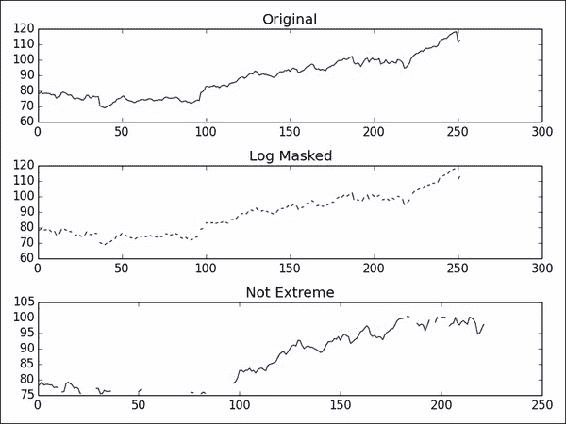
2. 让我们将极值定义为低于平均值的一个标准差，或高于平均值的一个标准差（这仅用于演示目的）。 编写以下代码以屏蔽极值：

   dev = close.std()
   avg = close.mean()
   inside = numpy.ma.masked_outside(close, avg - dev, avg + dev)
   print("Inside", inside[:10], "...")
   

   此代码显示前十个元素：

   Inside [-- -- -- -- -- -- 409.429675172 410.240597855 -- --] ...
   
   

   绘制原始价格数据，绘制对数后的数据，再次绘制指数，最后绘制基于标准差的遮罩后的数据。 以下屏幕截图显示了结果（此运行）：

   

   本教程的完整程序如下：

   from __future__ import print_function
   import numpy as np
   from matplotlib.finance import quotes_historical_yahoo
   from datetime import date
   import matplotlib.pyplot as plt
   def get_close(ticker):
      today = date.today()
      start = (today.year - 1, today.month, today.day)
   
      quotes = quotes_historical_yahoo(ticker, start, today)
   
      return np.array([q[4] for q in quotes])
   
   close = get_close('AAPL')
   
   triples = np.arange(0, len(close), 3)
   print("Triples", triples[:10], "...")
   
   signs = np.ones(len(close))
   print("Signs", signs[:10], "...")
   
   signs[triples] = -1
   print("Signs", signs[:10], "...")
   
   ma_log = np.ma.log(close * signs)
   print("Masked logs", ma_log[:10], "...")
   
   dev = close.std()
   avg = close.mean()
   inside = np.ma.masked_outside(close, avg - dev, avg + dev)
   print("Inside", inside[:10], "...")
   
   plt.subplot(311)
   plt.title("Original")
   plt.plot(close)
   
   plt.subplot(312)
   plt.title("Log Masked")
   plt.plot(np.exp(ma_log))
   
   plt.subplot(313)
   plt.title("Not Extreme")
   plt.plot(inside)
   
   plt.tight_layout()
   plt.show()
   

工作原理

numpy.ma模块中的函数掩盖了数组元素，我们认为这些元素是非法的。 例如，log()和sqrt()函数不允许使用负值。 屏蔽值类似于数据库和编程中的NULL或None值。 具有屏蔽值的所有操作都将导致屏蔽值。

另见

• numpy.ma模块的文档

使用recarray函数创建得分表

recarray类是ndarray的子类。 这些数组可以像数据库中一样保存记录，具有不同的数据类型。 例如，我们可以存储有关员工的记录，其中包含诸如薪水之类的数字数据和诸如员工姓名之类的字符串。

现代经济理论告诉我们，投资归结为优化风险和回报。 风险是由对数回报的标准差表示的。 另一方面，奖励由对数回报的平均值表示。 我们可以拿出相对分数，高分意味着低风险和高回报。 这只是理论上的，未经测试，所以不要太在意。 我们将计算几只股票的得分，并将它们与股票代号一起使用 NumPy recarray()函数中的表格格式存储。

操作步骤

让我们从创建记录数组开始：

1. 为每个记录创建一个包含符号，标准差得分，平均得分和总得分的记录数组：

   weights = np.recarray((len(tickers),), dtype=[('symbol', np.str_, 16), 
       ('stdscore', float), ('mean', float), ('score', float)])
   

2. 为了简单起见，请根据对数收益在循环中初始化得分：

   for i, ticker in enumerate(tickers):
      close = get_close(ticker)
      logrets = np.diff(np.log(close))
      weights[i]['symbol'] = ticker
      weights[i]['mean'] = logrets.mean()
      weights[i]['stdscore'] = 1/logrets.std()
      weights[i]['score'] = 0
   

   如您所见，我们可以使用在上一步中定义的字段名称来访问元素。

3. 现在，我们有一些数字，但是它们很难相互比较。 归一化分数，以便我们以后可以将它们合并。 在这里，归一化意味着确保分数加起来为：

   for key in ['mean', 'stdscore']:
       wsum = weights[key].sum()
       weights[key] = weights[key]/wsum
   

4. 总体分数将只是中间分数的平均值。 对总分上的记录进行排序以产生排名：

   weights['score'] = (weights['stdscore'] + weights['mean'])/2
   weights['score'].sort()
   

   The following is the complete code for this example:

   from __future__ import print_function
   import numpy as np
   from matplotlib.finance import quotes_historical_yahoo
   from datetime import date
   
   tickers = ['MRK', 'T', 'VZ']
   
   def get_close(ticker):
      today = date.today()
      start = (today.year - 1, today.month, today.day)
   
      quotes = quotes_historical_yahoo(ticker, start, today)
   
      return np.array([q[4] for q in quotes])
   
   weights = np.recarray((len(tickers),), dtype=[('symbol', np.str_, 16), 
      ('stdscore', float), ('mean', float), ('score', float)])
   
   for i, ticker in enumerate(tickers):
      close = get_close(ticker)
      logrets = np.diff(np.log(close))
      weights[i]['symbol'] = ticker
      weights[i]['mean'] = logrets.mean()
      weights[i]['stdscore'] = 1/logrets.std()
      weights[i]['score'] = 0
   
   for key in ['mean', 'stdscore']:
      wsum = weights[key].sum()
      weights[key] = weights[key]/wsum
   
   weights['score'] = (weights['stdscore'] + weights['mean'])/2
   weights['score'].sort()
   
   for record in weights:
      print("%s,mean=%.4f,stdscore=%.4f,score=%.4f" % (record['symbol'], record['mean'], record['stdscore'], record['score']))
   

   该程序产生以下输出：

   MRK,mean=0.8185,stdscore=0.2938,score=0.2177
   T,mean=0.0927,stdscore=0.3427,score=0.2262
   VZ,mean=0.0888,stdscore=0.3636,score=0.5561
   
   

分数已归一化，因此值介于0和1之间，我们尝试从秘籍开始使用定义获得最佳收益和风险组合 。 根据输出，VZ得分最高，因此是最好的投资。 当然，这只是一个 NumPy 演示，数据很少，所以不要认为这是推荐。

工作原理

我们计算了几只股票的得分，并将它们存储在recarray NumPy 对象中。 这个数组使我们能够混合不同数据类型的数据，在这种情况下，是股票代码和数字得分。 记录数组使我们可以将字段作为数组成员访问，例如arr.field。 本教程介绍了记录数组的创建。 您可以在numpy.recarray模块中找到更多与记录数组相关的功能。

另见

• numpy.recarray模块的文档