文章目录
- 1. 代码讲解
- 1.1 PatchEmbed类
- 1)`__init__ `函数
- 2) forward 过程
- 1.2 Attention类
- 1)`__init__ `函数
- 2)forward 过程
- 1.3 MLP类
- 1)`__init__ `函数
- 2)forward函数
- 1.4 Block类
- 1)`__init__ `函数
- 2)forward函数
- 1.5 Vision Transformer类
- 1)`__init__ `函数
- 2)forward 函数
- 1.6 构建各种版本的VIT模型
- 2. 使用介绍
- 参考
Vision Transformer(ViT) 的理论部分,参考我之前写的博文: Vision Transformer(ViT) 1: 理论详解
1. 代码讲解

网络详细介绍,参见博客: Vision Transformer(ViT) 1: 理论详解
模型构建的对应的代码在vit_transformer.py中:
1.1 PatchEmbed类
PatchEmbed类对应网络结构中PathEmbeding部分,它的结构很简单,由一个卷积核为16x16,步距为16的卷积实现。实现的代码如下:
class PatchEmbed(nn.Module):
    """
    2D Image to Patch Embedding
    """
    def __init__(self, img_size=224, patch_size=16, in_c=3, embed_dim=768, norm_layer=None):
        super().__init__()
        img_size = (img_size, img_size)
        patch_size = (patch_size, patch_size)
        self.img_size = img_size
        self.patch_size = patch_size
        self.grid_size = (img_size[0] // patch_size[0], img_size[1] // patch_size[1])
        self.num_patches = self.grid_size[0] * self.grid_size[1]

        self.proj = nn.Conv2d(in_c, embed_dim, kernel_size=patch_size, stride=patch_size)
        self.norm = norm_layer(embed_dim) if norm_layer else nn.Identity()

    def forward(self, x):
        B, C, H, W = x.shape
        assert H == self.img_size[0] and W == self.img_size[1], \
            f"Input image size ({H}*{W}) doesn't match model ({self.img_size[0]}*{self.img_size[1]})."

        # flatten: [B, C, H, W] -> [B, C, HW]
        # transpose: [B, C, HW] -> [B, HW, C]
        x = self.proj(x).flatten(2).transpose(1, 2)
        x = self.norm(x)
        return x
1)__init__ 函数
- 在初始化
__init__函数中,由于传入的是RGB3通道图片,因此in_c=3(in_channel);
针对VIT-B/16模型中embed_dim=768; 参数norm_layer默认为None. num_patches等于经16x16卷积后得到的featuremap进行展平: 14 x14。定义卷积层,kernel_size为16x16,stride为16,输入channel为in_c,输出channel为embed_dim为196, 针对VIT-L/16或其他的类型embed_dim值是有变化的。
self.proj = nn.Conv2d(in_c, embed_dim, kernel_size=patch_size, stride=patch_size)
norm_layer默认是为None的,如果有传入norm_layer就会初始化norm_layer。如果为None,self.norm则为nn.Identity()也就是不做任何操作
2) forward 过程
- 首先判断传入的图片尺寸是否等于预先设定的尺寸,如果不是则会报错。需要
注意的是:VIT模型不像传统的CNN模型是可以更改输入尺寸的。在我们VIT模型输入图片尺寸必须是固定的。 - 接下来将数据输入卷积层,得到shape为
[ B C H W]的tensor, 然后对宽和高进行展平处理得到shape为[ B C HW], 然后再用transpose交换维度1,2的顺序,最终得到shape为[B HW C]
# flatten: [B, C, H, W] -> [B, C, HW]
# transpose: [B, C, HW] -> [B, HW, C]
x = self.proj(x).flatten(2).transpose(1, 2)
- 最后将结果通过LayerNorm进行输出。
1.2 Attention类
Attention类就是实现多头自注意力模块(multi head self attention),完整的代码如下:
class Attention(nn.Module):
    def __init__(self,
                 dim,   # 输入token的dim
                 num_heads=8,
                 qkv_bias=False,
                 qk_scale=None,
                 attn_drop_ratio=0.,
                 proj_drop_ratio=0.):
        super(Attention, self).__init__()
        self.num_heads = num_heads
        head_dim = dim // num_heads
        self.scale = qk_scale or head_dim ** -0.5
        self.qkv = nn.Linear(dim, dim * 3, bias=qkv_bias)
        self.attn_drop = nn.Dropout(attn_drop_ratio)
        self.proj = nn.Linear(dim, dim)
        self.proj_drop = nn.Dropout(proj_drop_ratio)

    def forward(self, x):
        # [batch_size, num_patches + 1, total_embed_dim]
        B, N, C = x.shape

        # qkv(): -> [batch_size, num_patches + 1, 3 * total_embed_dim]
        # reshape: -> [batch_size, num_patches + 1, 3, num_heads, embed_dim_per_head]
        # permute: -> [3, batch_size, num_heads, num_patches + 1, embed_dim_per_head]
        qkv = self.qkv(x).reshape(B, N, 3, self.num_heads, C // self.num_heads).permute(2, 0, 3, 1, 4)
        # [batch_size, num_heads, num_patches + 1, embed_dim_per_head]
        q, k, v = qkv[0], qkv[1], qkv[2]  # make torchscript happy (cannot use tensor as tuple)

        # transpose: -> [batch_size, num_heads, embed_dim_per_head, num_patches + 1]
        # @: multiply -> [batch_size, num_heads, num_patches + 1, num_patches + 1]
        attn = (q @ k.transpose(-2, -1)) * self.scale
        attn = attn.softmax(dim=-1)
        attn = self.attn_drop(attn)

        # @: multiply -> [batch_size, num_heads, num_patches + 1, embed_dim_per_head]
        # transpose: -> [batch_size, num_patches + 1, num_heads, embed_dim_per_head]
        # reshape: -> [batch_size, num_patches + 1, total_embed_dim]
        x = (attn @ v).transpose(1, 2).reshape(B, N, C)
        x = self.proj(x)
        x = self.proj_drop(x)
        return x
1)__init__ 函数
- dim 参数代表的是
embed_dim,也就是输入token的dim;num_head指的是multi head self attention模块的head数目;qkv_bias指的是生成qkv的时候,是否去使用偏执bias,默认是为False,如果为True的话就会使用该偏执;qk_sclae是计算qk的缩放因子。 head_dim:针对每个head的dimension,就等于dim // num_head。self_scale: 如果有传入qk_scale的话:self_scale = qk_scale,如果没有传入就等于 1 h e a d _ d i m \frac{1}{\sqrt{head\_dim}} head_dim1,参考如下公式:

qkv在网络中是通过全连接进行计算得到的,值得注意的是有些源码是通过3个全连接层分别得到q,k,v,但我们这里使用一个节点数为3*dim的全连接层,一次性得到qkv,其实这两种方式都是可以的。
self.qkv = nn.Linear(dim, dim * 3, bias=qkv_bias)
- 然后再定义一个
drop_out层 - 紧接着,再定义一个全连接层
nn.Linear。因为在multi head self attention的理论中,会将各个head的结果进行concat拼接,然后通过与 W o W^o Wo相乘进行映射,这里就可以利用全连接来实现。
self.proj = nn.Linear(dim, dim)
- 接下来,再定义一个
Drop out层。
2)forward 过程
- 正向传播的输入tensor
x的shape大小为[batch_size,num_patches+1,total_embed_dim],这里的num_patches等于196,这里+1是因为加上了一个class_token - 然后利用
全连接,计算qkv的值
# qkv(): -> [batch_size, num_patches + 1, 3 * total_embed_dim]
# reshape: -> [batch_size, num_patches + 1, 3, num_heads, embed_dim_per_head]
# permute: -> [3, batch_size, num_heads, num_patches + 1, embed_dim_per_head]
qkv = self.qkv(x).reshape(B, N, 3, self.num_heads, C // self.num_heads).permute(2, 0, 3, 1, 4)
# [batch_size, num_heads, num_patches + 1, embed_dim_per_head]
q, k, v = qkv[0], qkv[1], qkv[2]  # make torchscript happy (cannot use tensor as tuple)
- 然后将
q,k矩阵相乘,并乘以scale,再经过softmax计算,就计算得到针对每个v的权重,最后将结果与V矩阵相乘:整个过程就是实现如下公式的计算。

attn = (q @ k.transpose(-2, -1)) * self.scale
attn = attn.softmax(dim=-1)
attn = self.attn_drop(attn)

# @: multiply -> [batch_size, num_heads, num_patches + 1, embed_dim_per_head]
# transpose: -> [batch_size, num_patches + 1, num_heads, embed_dim_per_head]
# reshape: -> [batch_size, num_patches + 1, total_embed_dim]
x = (attn @ v).transpose(1, 2).reshape(B, N, C)
需要将每个head的结果进行concat拼接,这里通过reshape(B,N,C)实现,将shape由[batch_size, num_patches + 1, num_heads, embed_dim_per_head]转为[batch_size, num_patches + 1, total_embed_dim], 其中total_embed_dim = num_heads,*embed_dim_per_head
- 然后将结果通过 W o W^o Wo进行映射,通过这里的全连接实现。
x = self.proj(x)
- 最后通过drop_out层,得到multi head self atention的输出。
以上就是Attention类的实现过程。
1.3 MLP类
MLP 指的是Encoder Block中的MLP Block,结构比较简单。首先是一个全连接层,然后加上GELU激活函数,然后Droupout, 然后再全连接层,最后通过一个Dropout进行全连接层输出。

完整的实现代码如下:
class Mlp(nn.Module):
    """
    MLP as used in Vision Transformer, MLP-Mixer and related networks
    """
    def __init__(self, in_features, hidden_features=None, out_features=None, act_layer=nn.GELU, drop=0.):
        super().__init__()
        out_features = out_features or in_features
        hidden_features = hidden_features or in_features
        self.fc1 = nn.Linear(in_features, hidden_features)
        self.act = act_layer()
        self.fc2 = nn.Linear(hidden_features, out_features)
        self.drop = nn.Dropout(drop)

    def forward(self, x):
        x = self.fc1(x)
        x = self.act(x)
        x = self.drop(x)
        x = self.fc2(x)
        x = self.drop(x)
        return x
在:Vision Transformer(ViT) 1: 理论详解中有讲到过,第一个全连接层Linear的节点个数是输入节点个数的4倍,第二个全连接层会将节点个数还原回我们输入的节点个数。
1)__init__ 函数
- 在初始化函数中,会传入
in_features(输入节点个数);hidden_features(第一个全连接层的节点个数),一般是in_features的4倍;out_features其实和in_features是一样的。这里还有个激活函数,默认是nn.GELU激活函数。 - 如果有传入
out_features,则out_features为传入的out_features,如果没有传入则等于in_features; 同样,hidden_features如果传入hidden_features,则等于hidden_features,如果没有传入则等于in_features。 - 接下来定义全连接层1,激活函数,全连接层2,以及最后的
Dropout
2)forward函数
将输入一次传给全连接层1,激活函数,dropout,全连接层2,dropout层
1.4 Block类
这里定义的Block就是结构中的Encoder Block; 在Transforer Encoder层,就是将Encoder Block重复堆叠L次。Block类实现的Encoder Block网络结构如下:

Encoder Block 首先会通过Layer Norm,然后Multi-Head Attention,再接上Drouput层,然后再通过捷径分支进行相加,然后再通过Layer Norm和MLP Block以及Droupout层, 然后再通过一个捷径分支相加,得到Encoder Block的最终输出。 完整的实现代码如下:
class Block(nn.Module):
    def __init__(self,
                 dim,
                 num_heads,
                 mlp_ratio=4.,
                 qkv_bias=False,
                 qk_scale=None,
                 drop_ratio=0.,
                 attn_drop_ratio=0.,
                 drop_path_ratio=0.,
                 act_layer=nn.GELU,
                 norm_layer=nn.LayerNorm):
        super(Block, self).__init__()
        self.norm1 = norm_layer(dim)
        self.attn = Attention(dim, num_heads=num_heads, qkv_bias=qkv_bias, qk_scale=qk_scale,
                              attn_drop_ratio=attn_drop_ratio, proj_drop_ratio=drop_ratio)
        # NOTE: drop path for stochastic depth, we shall see if this is better than dropout here
        self.drop_path = DropPath(drop_path_ratio) if drop_path_ratio > 0. else nn.Identity()
        self.norm2 = norm_layer(dim)
        mlp_hidden_dim = int(dim * mlp_ratio)
        self.mlp = Mlp(in_features=dim, hidden_features=mlp_hidden_dim, act_layer=act_layer, drop=drop_ratio)

    def forward(self, x):
        x = x + self.drop_path(self.attn(self.norm1(x)))
        x = x + self.drop_path(self.mlp(self.norm2(x)))
        return x
1)__init__ 函数
dim对应每个token的dimension;num_heads就是multi head attention中使用的head个数;mlp_ratio默认为4,定义了第一个全连接层的节点数是输入节点个数的4倍。qkv_bias默认为False,不使用bias。- 定义了
norm1层以及multi head attention结构,通过调用Attention类实现。 - 如果传入的
drop_path_ratio大于0,就会实例化一个DropPath方法。如果条件不满足就会使用nn.Identity也就是不进行任何操作 - 接下来定义
norm2,然后计算mlp_hidden_dim也就是第一个全连接层节点数:mlp_hidden_dim = int(dim * mlp_ratio) - 然后再初始化
MLP Block参数,通过调用Block类来实例化
2)forward函数
正向传播过程
- 输入x首先通过norm1,
multi head self attention以及drop_path,然后再加上我们的输入x进行shortcut相加,得到第一个捷径分支的输出x - 接下来,再将我们的结果依次通过
norm2,mlp和drop_path,然后和上面得到的x进行Add相加,得到最终的输出。
1.5 Vision Transformer类
Vision Transformer类,利用之前定义好的各个模块,实现完整的Vison Transformer结构

ViT-B/16的完整代码实现,如下:
class VisionTransformer(nn.Module):
    def __init__(self, img_size=224, patch_size=16, in_c=3, num_classes=1000,
                 embed_dim=768, depth=12, num_heads=12, mlp_ratio=4.0, qkv_bias=True,
                 qk_scale=None, representation_size=None, distilled=False, drop_ratio=0.,
                 attn_drop_ratio=0., drop_path_ratio=0., embed_layer=PatchEmbed, norm_layer=None,
                 act_layer=None):

        super(VisionTransformer, self).__init__()
        self.num_classes = num_classes
        self.num_features = self.embed_dim = embed_dim  # num_features for consistency with other models
        self.num_tokens = 2 if distilled else 1
        norm_layer = norm_layer or partial(nn.LayerNorm, eps=1e-6)
        act_layer = act_layer or nn.GELU

        self.patch_embed = embed_layer(img_size=img_size, patch_size=patch_size, in_c=in_c, embed_dim=embed_dim)
        num_patches = self.patch_embed.num_patches

        self.cls_token = nn.Parameter(torch.zeros(1, 1, embed_dim))
        self.dist_token = nn.Parameter(torch.zeros(1, 1, embed_dim)) if distilled else None
        self.pos_embed = nn.Parameter(torch.zeros(1, num_patches + self.num_tokens, embed_dim))
        self.pos_drop = nn.Dropout(p=drop_ratio)

        dpr = [x.item() for x in torch.linspace(0, drop_path_ratio, depth)]  # stochastic depth decay rule
        self.blocks = nn.Sequential(*[
            Block(dim=embed_dim, num_heads=num_heads, mlp_ratio=mlp_ratio, qkv_bias=qkv_bias, qk_scale=qk_scale,
                  drop_ratio=drop_ratio, attn_drop_ratio=attn_drop_ratio, drop_path_ratio=dpr[i],
                  norm_layer=norm_layer, act_layer=act_layer)
            for i in range(depth)
        ])
        self.norm = norm_layer(embed_dim)

        # Representation layer
        if representation_size and not distilled:
            self.has_logits = True
            self.num_features = representation_size
            self.pre_logits = nn.Sequential(OrderedDict([
                ("fc", nn.Linear(embed_dim, representation_size)),
                ("act", nn.Tanh())
            ]))
        else:
            self.has_logits = False
            self.pre_logits = nn.Identity()

        # Classifier head(s)
        self.head = nn.Linear(self.num_features, num_classes) if num_classes > 0 else nn.Identity()
        self.head_dist = None
        if distilled:
            self.head_dist = nn.Linear(self.embed_dim, self.num_classes) if num_classes > 0 else nn.Identity()

        # Weight init
        nn.init.trunc_normal_(self.pos_embed, std=0.02)
        if self.dist_token is not None:
            nn.init.trunc_normal_(self.dist_token, std=0.02)

        nn.init.trunc_normal_(self.cls_token, std=0.02)
        self.apply(_init_vit_weights)

    def forward_features(self, x):
        # [B, C, H, W] -> [B, num_patches, embed_dim]
        x = self.patch_embed(x)  # [B, 196, 768]
        # [1, 1, 768] -> [B, 1, 768]
        cls_token = self.cls_token.expand(x.shape[0], -1, -1)
        if self.dist_token is None:
            x = torch.cat((cls_token, x), dim=1)  # [B, 197, 768]
        else:
            x = torch.cat((cls_token, self.dist_token.expand(x.shape[0], -1, -1), x), dim=1)

        x = self.pos_drop(x + self.pos_embed)
        x = self.blocks(x)
        x = self.norm(x)
        if self.dist_token is None:
            return self.pre_logits(x[:, 0])
        else:
            return x[:, 0], x[:, 1]

    def forward(self, x):
        x = self.forward_features(x)
        if self.head_dist is not None:
            x, x_dist = self.head(x[0]), self.head_dist(x[1])
            if self.training and not torch.jit.is_scripting():
                # during inference, return the average of both classifier predictions
                return x, x_dist
            else:
                return (x + x_dist) / 2
        else:
            x = self.head(x)
        return x
1)__init__ 函数
- 可以看到在
__init__初始化函数中传入了很多参数。 - 首先是
img_size,默认是224x224;patch_size默认为16,in_c(in_channel)默认为3;num_classes默认为1000;embed_dim默认为768;depth默认为12,depth指的是在Transformer Encoder中重复堆叠Encoder Block的次数。representation_size对应的分类预测层MLP head中的Pre_Logits中全连接层的节点个数,representation_size默认为None,如果为None的话就不会构建MLP Head当中的Pre_Logits,此时在MLP Head中只有一个全连接层;distilled参数可以不用管,因为作者是为了搭建DeiT模型使用的。embed_layer对应embeding层,默认使用PatchEmbed层结构。 - 由于
distilled在`VIT模型中是用不到的,所以我们的num_token为1 (class_token) - 通过
PatchEmbed实例化构建patch_embed,传入img_size,patch_size以及in_c和embed_dim参数,就构建好了PatchEmbed层。 - 接下来,需要加上一个
class token它的shape为(1,768);class_token会和Patch Embeding的输出进行Concat相加。这里初始化了一个shape为(1,1,768)零矩阵,来定义cls_token,其中shape的第一个维度1,对应的是batch维度。
self.cls_token = nn.Parameter(torch.zeros(1, 1, embed_dim))
dist_token在VIT模型是使用不到的,distilled为False,对应dist_token为None- 接下来定义位置编码
pos_embed, 其中pos_embed是和concat拼接后的shape是一样的,对应VIT-B/16模型,它的shape就是(197,768)。 这里通过nn.Parameter创建一个可训练的参数,使用零矩阵进行初始化,shape大小为(1,num_patches+self.num_tokens,embed_dim),其中第一个维度1为batch维,可以不用管。 - 接下来,根据传入的
drop_path_ratio, 构造一个长度depth,从0到drop_path_ratio范围等差变化。也就是说在Transformer Encoder中每一个Encoder Block它们所采用的drop_path方法,使用的drop_path_ratio是递增的。 - 然后构建
Transormer Encoder模块,重复堆叠Encoder BlockL次。通过nn.Sequential方法将循环创建depth次的Block(Encoder Block)打包为一个整体。这样就创建好了Transormer Encoder模块,变量名为blocks。
 self.blocks = nn.Sequential(*[
            Block(dim=embed_dim, num_heads=num_heads, mlp_ratio=mlp_ratio, qkv_bias=qkv_bias, qk_scale=qk_scale,
                  drop_ratio=drop_ratio, attn_drop_ratio=attn_drop_ratio, drop_path_ratio=dpr[i],
                  norm_layer=norm_layer, act_layer=act_layer)
            for i in range(depth)
        ])
- 接下来,再构建一个
norm_layer, 作用于Transormer Encoder模块后。 - 构建pre_logits层:如果
representation_size有值的话,就将has_logits参数设置为True,并将representation_size赋值给num_features。然后利用nn.Sequential构建pre_logits层,它就是一个全连接层fc+ nn.Tanh()激活函数;如果representation_size为None的话,has_logits参数就为False。pre_logits就等于nn.Identity()也就是不做任何处理,相当于没有pre_logits层。 - 接下来,构建
Classifier Head,通过一个全连接层实现,输入的节点为num_features,输出为分类个数num_classes。
2)forward 函数
forward函数的代码实现如下:
def forward(self, x):
        x = self.forward_features(x)
        if self.head_dist is not None:
            x, x_dist = self.head(x[0]), self.head_dist(x[1])
            if self.training and not torch.jit.is_scripting():
                # during inference, return the average of both classifier predictions
                return x, x_dist
            else:
                return (x + x_dist) / 2
        else:
            x = self.head(x)
        return x
正向传播过程
- 首先会将x传入给forward_feature,对应的forwar_feature实现如下:
  def forward_features(self, x):
       # [B, C, H, W] -> [B, num_patches, embed_dim]
       x = self.patch_embed(x)  # [B, 196, 768]
       # [1, 1, 768] -> [B, 1, 768]
       cls_token = self.cls_token.expand(x.shape[0], -1, -1)
       if self.dist_token is None:
           x = torch.cat((cls_token, x), dim=1)  # [B, 197, 768]
       else:
           x = torch.cat((cls_token, self.dist_token.expand(x.shape[0], -1, -1), x), dim=1)

       x = self.pos_drop(x + self.pos_embed)
       x = self.blocks(x)
       x = self.norm(x)
       if self.dist_token is None:
           return self.pre_logits(x[:, 0])
       else:
           return x[:, 0], x[:, 1]
- 首先将输入传入给
patch_embed, - 然后将
cls_token通过expand方法由shape为[1,1,768], expand到(batch_size,196,768), 再将cls_token与patch_embed的输出进行concat拼接。 - 然后将
concat之后的x加上pos_embed(位置编码),shape变为(batch_size,197,768) - 紧接着再通过一个
dropout层 - 然后再将数据传给blocks,也就是我们定义好的
Transformer Encoder层 - 然后再通过
Layer_Norm层 - 然后提取class_token输出,通过x[:,0]取197中的第一个token, 然后将取出来的数据传入给
pre_logits,之前我们说到过如果representation_size为None的话,就是一个Identity层,它会直接返回cls_token作为输出。
再回到forward函数中,由于head_dist参数为None, 因此会执行到x = self.head(x)中。head对应的就是Classifier Head,用于最后分类的全连接层。以上就是整个VIT模型的搭建过程。
1.6 构建各种版本的VIT模型
根据不同的VIT配合,搭建对应的VIT模型。
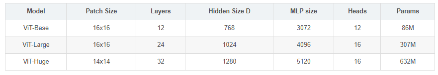
在论文的Table1中有给出三个模型(Base/ Large/ Huge)的参数,在源码中除了有Patch Size为16x16的外还有32x32的。其中的Layers就是Transformer Encoder中重复堆叠Encoder Block的次数,Hidden Size就是对应通过Embedding层后每个token的dim(向量的长度),MLP size是Transformer Encoder中MLP Block第一个全连接的节点个数(是Hidden Size的4倍),Heads代表Transformer中Multi-Head Attention的heads数。
(2) 构建ViT-B/16模型
def vit_base_patch32_224(num_classes: int = 1000):
    """
    ViT-Base model (ViT-B/32) from original paper (https://arxiv.org/abs/2010.11929).
    ImageNet-1k weights @ 224x224, source https://github.com/google-research/vision_transformer.
    weights ported from official Google JAX impl:
    链接: https://pan.baidu.com/s/1hCv0U8pQomwAtHBYc4hmZg  密码: s5hl
    """
    model = VisionTransformer(img_size=224,
                              patch_size=32,
                              embed_dim=768,
                              depth=12,
                              num_heads=12,
                              representation_size=None,
                              num_classes=num_classes)
    return model
(2) 构建ViT-B/16 在imagenet21k上预训练的模型
def vit_base_patch16_224_in21k(num_classes: int = 21843, has_logits: bool = True):
    """
    ViT-Base model (ViT-B/16) from original paper (https://arxiv.org/abs/2010.11929).
    ImageNet-21k weights @ 224x224, source https://github.com/google-research/vision_transformer.
    weights ported from official Google JAX impl:
    https://github.com/rwightman/pytorch-image-models/releases/download/v0.1-vitjx/jx_vit_base_patch16_224_in21k-e5005f0a.pth
    """
    model = VisionTransformer(img_size=224,
                              patch_size=16,
                              embed_dim=768,
                              depth=12,
                              num_heads=12,
                              representation_size=768 if has_logits else None,
                              num_classes=num_classes)
    return model
num_classes:21843,代表imagenet21k的分类个数has_logits为True,表示使用了pred_logits层
(3) 构建ViT-B/32 在imagenet21k上预训练的模型
def vit_base_patch32_224_in21k(num_classes: int = 21843, has_logits: bool = True):
    """
    ViT-Base model (ViT-B/32) from original paper (https://arxiv.org/abs/2010.11929).
    ImageNet-21k weights @ 224x224, source https://github.com/google-research/vision_transformer.
    weights ported from official Google JAX impl:
    https://github.com/rwightman/pytorch-image-models/releases/download/v0.1-vitjx/jx_vit_base_patch32_224_in21k-8db57226.pth
    """
    model = VisionTransformer(img_size=224,
                              patch_size=32,
                              embed_dim=768,
                              depth=12,
                              num_heads=12,
                              representation_size=768 if has_logits else None,
                              num_classes=num_classes)
    return model
(3) 构建ViT-L/16模型
ef vit_large_patch16_224(num_classes: int = 1000):
    """
    ViT-Large model (ViT-L/16) from original paper (https://arxiv.org/abs/2010.11929).
    ImageNet-1k weights @ 224x224, source https://github.com/google-research/vision_transformer.
    weights ported from official Google JAX impl:
    链接: https://pan.baidu.com/s/1cxBgZJJ6qUWPSBNcE4TdRQ  密码: qqt8
    """
    model = VisionTransformer(img_size=224,
                              patch_size=16,
                              embed_dim=1024,
                              depth=24,
                              num_heads=16,
                              representation_size=None,
                              num_classes=num_classes)
    return model
embed_dim:相对于VIT-B的768,增大到1024depth: 相对于VIT-B的12,增大到24num_heads: 相对于VIT-B的12,增大到16
(4) 构建ViT-L/16 在imagenet21k上预训练的模型
def vit_large_patch16_224_in21k(num_classes: int = 21843, has_logits: bool = True):
    """
    ViT-Large model (ViT-L/16) from original paper (https://arxiv.org/abs/2010.11929).
    ImageNet-21k weights @ 224x224, source https://github.com/google-research/vision_transformer.
    weights ported from official Google JAX impl:
    https://github.com/rwightman/pytorch-image-models/releases/download/v0.1-vitjx/jx_vit_large_patch16_224_in21k-606da67d.pth
    """
    model = VisionTransformer(img_size=224,
                              patch_size=16,
                              embed_dim=1024,
                              depth=24,
                              num_heads=16,
                              representation_size=1024 if has_logits else None,
                              num_classes=num_classes)
    return model
(5) 构建ViT-L/32 在imagenet21k上预训练的模型
def vit_large_patch32_224_in21k(num_classes: int = 21843, has_logits: bool = True):
    """
    ViT-Large model (ViT-L/32) from original paper (https://arxiv.org/abs/2010.11929).
    ImageNet-21k weights @ 224x224, source https://github.com/google-research/vision_transformer.
    weights ported from official Google JAX impl:
    https://github.com/rwightman/pytorch-image-models/releases/download/v0.1-vitjx/jx_vit_large_patch32_224_in21k-9046d2e7.pth
    """
    model = VisionTransformer(img_size=224,
                              patch_size=32,
                              embed_dim=1024,
                              depth=24,
                              num_heads=16,
                              representation_size=1024 if has_logits else None,
                              num_classes=num_classes)
    return model
(6) 构建ViT-H/14 在imagenet21k上预训练的模型
def vit_huge_patch14_224_in21k(num_classes: int = 21843, has_logits: bool = True):
    """
    ViT-Huge model (ViT-H/14) from original paper (https://arxiv.org/abs/2010.11929).
    ImageNet-21k weights @ 224x224, source https://github.com/google-research/vision_transformer.
    NOTE: converted weights not currently available, too large for github release hosting.
    """
    model = VisionTransformer(img_size=224,
                              patch_size=14,
                              embed_dim=1280,
                              depth=32,
                              num_heads=16,
                              representation_size=1280 if has_logits else None,
                              num_classes=num_classes)
    return model
patch_size:为14x14,不是原来的16x16embed_dim:是1280depth: 为32
不建议使用VIT-H/14,因为模型太大了,下载预训练权重就有将近1个G, 这里不同模型都给出了预训练权重的下载链接 .
建议大家在训练的时候,使用预训练权重,对于VIT模型如果不使用预训练权重,它的效果示很差的。原论文指出,VIT模型直接在imagenet上预训练,其他它的效果其实并不好,它只有在非常大的数据集训练之后,才会有比较好的效果。所以建议使用预训练权重,进行迁移学习训练。
2. 使用介绍
- (1)下载好数据集,代码中默认使用的是花分类数据集,下载地址: https://storage.googleapis.com/download.tensorflow.org/example_images/flower_photos.tgz, 如果下载不了的话可以通过百度云链接下载: https://pan.baidu.com/s/1QLCTA4sXnQAw_yvxPj9szg 提取码:58p0
- (2)在
train.py脚本中将--data-path设置成解压后的flower_photos文件夹绝对路径 - (3)下载预训练权重,在
vit_model.py文件中每个模型都有提供预训练权重的下载地址,根据自己使用的模型下载对应预训练权重 - (4)在
train.py脚本中将--weights参数设成下载好的预训练权重路径 - (5)设置好数据集的路径
--data-path以及预训练权重的路径--weights就能使用train.py脚本开始训练了(训练过程中会自动生成class_indices.json文件) - (6)在
predict.py脚本中导入和训练脚本中同样的模型,并将model_weight_path设置成训练好的模型权重路径(默认保存在weights文件夹下) - (7)在
predict.py脚本中将img_path设置成你自己需要预测的图片绝对路径 - (8)设置好权重路径
model_weight_path和预测的图片路径img_path就能使用predict.py脚本进行预测了 - (9)如果要使用自己的数据集,请按照花分类数据集的文件结构进行摆放(即一个类别对应一个文件夹),并且将训练以及预测脚本中的num_classes设置成你自己数据的类别数
完整代码:
参考
1. Vision Transformer详解
2.Group Normalization详解
3. Layer Normalization解析