需要数据集和源码请点赞关注收藏后评论区留言~~~
一、生成对抗网络(GAN)
GAN(生成对抗网络)是用于教授DL模型以捕获训练数据分布的框架,因此可以从同一分布中生成新数据。它们由两个不同的模型组成,生成器和判别器。生成器的工作是生成看起来像训练图像的假图像,判别器的工作是查看图像并从生成器输出它是真实地训练图像还是伪图像。在训练过程中,生成器不断尝试通过生成越来越好地伪造品而使判别器的性能从超过智者,而判别器正在努力成为更好的侦探并正确的对真实和伪造图像进行分类。博弈的平衡点是当生成器生成的伪造品看起来像直接来自训练数据时,而判别器则始终猜测生成器输出是真实地还是伪造品地百分之五十置信度
二、DCGAN介绍
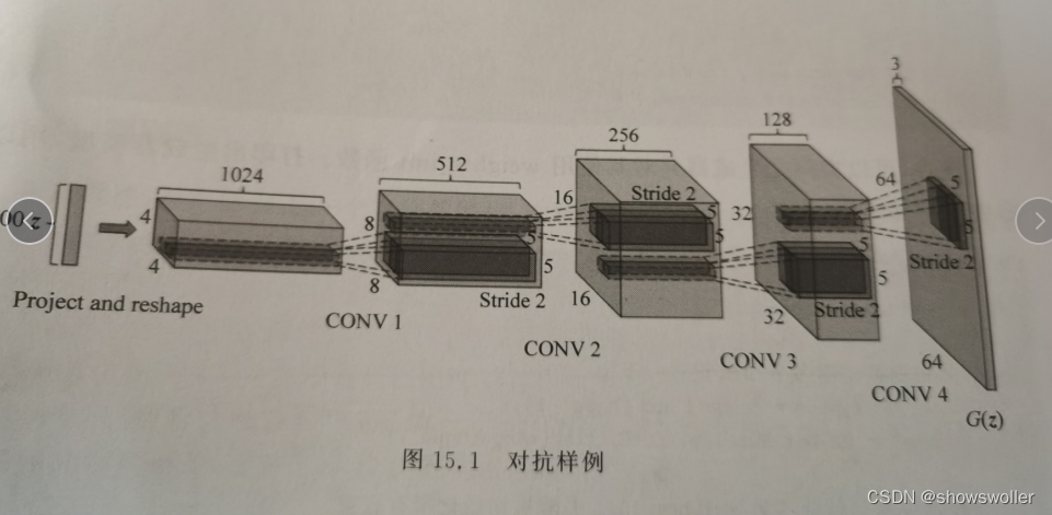
DCGAN是对上述GAN的直接扩展,除了它分别在判别器和生成器中明确地使用卷积和卷积转置层。判别器由卷积层、批标准化层以及LeakyReLU激活层组成,输入是3×64×64的图像,输出是输入图像来自实际数据的概率。生成器由转置卷积层,批标准化层以及ReLU激活层组成,输入是一个本征向量Z,它是从标准正太分别中采样得到的,输出是一个3×64×64的RGB图像
三、数据集简介
本篇博客用的数据集来自香港中文大学,名为img_align_celeba.zip 下载网址如下
数据集网址
由于访问不稳定以及文件过大 建议后台私信找我要
四、模型实现
1:权重初始化
所有模型权重均应从 mean=0 stdev=0.02的正太分别中随机初始化
2:生成器
生成器G用于将本征向量Z映射到数据空间
3:判别器
判别器D是一个二分类网络,它将图像作为输入并输出输入图像是真实的概率
4:损失函数和优化器
五、结果与可视化
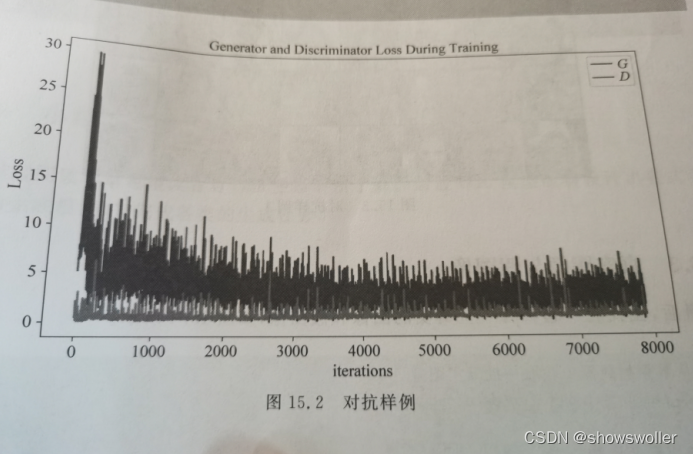
1:损失与训练迭代次数关系图
生成器和判别器的损失和训练迭代次数关系图如下
2:生成器G的训练进度
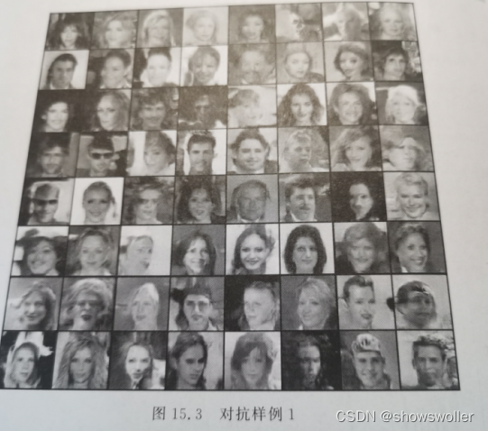
在每一个批次训练完成之后都保存了生成器的输出,现在可以通过动画可视化生成器G的训练进度
3:真实图像与假图像
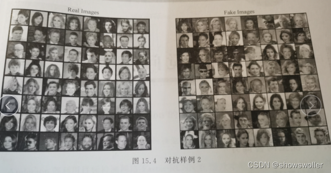
生成的假图像与真实图像对比如下
六、代码
部分源码如下
from __future__ import print_function
# %matplotlib inline
import argparse
import os
import random
import torch
import torch.nn as nn

hvision.transforms as transforms
import torchvision.utils as vutils
import numpy as np
import matplotlib.pyplot as plt
import matplotlib.animation as animation
from IPython.display import HTML

# Set random seed for reproducibility
manualSeed = 999
# manualSeed = random.randint(1, 10000) # use if you want new results
print("Random Seed: ", manualSeed)
random.seed(manualSeed)
torch.manual_seed(manualSeed)

# Inputs
# ------
#
# Let’s define some inputs for the run:
#
# -  **dataroot** - the path to the root of the dataset folder. We will
#    talk more about the dataset in the next section
# -  **workers** - the number of worker threads for loading the data with
#    the DataLoader
# -  **batch_size** - the batch size used in training. The DCGAN paper
#    uses a batch size of 128
# -  **image_size** - the spatial size of the images used for training.
#    This implementation defaults to 64x64. If another size is desired,
#    the structures of D and G must be changed. See
#    `here <https://github.com/pytorch/examples/issues/70>`__ for more
#    details
# -  **nc** - number of color channels in the input images. For color
#    images this is 3
# -  **nz** - length of latent vector
# -  **ngf** - relates to the depth of feature maps carried through the
#    generator
# -  **ndf** - sets the depth of feature maps propagated through the
#    discriminator
# -  **num_epochs** - number of training epochs to run. Training for
#    longer will probably lead to better results but will also take much
#    longer
# -  **lr** - learning rate for training. As described in the DCGAN paper,
#    this number should be 0.0002
# -  **beta1** - beta1 hyperparameter for Adam optimizers. As described in
#    paper, this number should be 0.5
# -  **ngpu** - number of GPUs available. If this is 0, code will run in
#    CPU mode. If this number is greater than 0 it will run on that number
#    of GPUs
#
#
#

# In[ ]:


# Root directory for dataset
dataroot = r"C:\Users\Admin\Desktop\celeba\img_align_celeba"

# Number of workers for dataloader
workers = 2

# Batch size during training
batch_size = 128

# Spatial size of training images. All images will be resized to this
#   size using a transformer.
image_size = 64

# Number of channels in the training images. For color images this is 3
nc = 3

# Size of z latent vector (i.e. size of generator input)
nz = 100

# Size of feature maps in generator
ngf = 64

# Size of feature maps in discriminator
ndf = 64

# Number of training epochs
num_epochs = 5

# Learning rate for optimizers
lr = 0.0002

# Beta1 hyperparam for Adam optimizers
beta1 = 0.5

# Number of GPUs available. Use 0 for CPU mode.
ngpu = 1

# Data
# ----
#
# In this tutorial we will use the `Celeb-A Faces
# dataset <http://mmlab.ie.cuhk.edu.hk/projects/CelebA.html>`__ which can
# be downloaded at the linked site, or in `Google
# Drive <https://drive.google.com/drive/folders/0B7EVK8r0v71pTUZsaXdaSnZBZzg>`__.
# The dataset will download as a file named *img_align_celeba.zip*. Once
# downloaded, create a directory named *celeba* and extract the zip file
# into that directory. Then, set the *dataroot* input for this notebook to
# the *celeba* directory you just created. The resulting directory
# structure should be:
#
# ::
#
#    /path/to/celeba
#        -> img_align_celeba
#            -> 188242.jpg
#            -> 173822.jpg
#            -> 284702.jpg
#            -> 537394.jpg
#               ...
#
# This is an important step because we will be using the ImageFolder
# dataset class, which requires there to be subdirectories in the
# dataset’s root folder. Now, we can create the dataset, create the
# dataloader, set the device to run on, and finally visualize some of the
# training data.
#
#
#

# In[ ]:


# We can use an image folder dataset the way we have it setup.
# Create the dataset
dataset = dset.ImageFolder(root=dataroot,
                           transform=transforms.Compose([
                               transforms.Resize(image_size),
                               transforms.CenterCrop(image_size),
                               transforms.ToTensor(),
                               transforms.Normalize((0.5, 0.5, 0.5), (0.5, 0.5, 0.5)),
                           ]))
# Create the dataloader
dataloader = torch.utils.data.DataLoader(dataset, batch_size=batch_size,
                                         shuffle=True, num_workers=workers)

# Decide which device we want to run on
device = torch.device("cuda:0" if (torch.cuda.is_available() and ngpu > 0) else "cpu")

# Plot some training images
real_batch = next(iter(dataloader))
plt.figure(figsize=(8, 8))
plt.axis("off")
plt.title("Training Images")
plt.imshow(np.transpose(vutils.make_grid(real_batch[0].to(device)[:64], padding=2, normalize=True).cpu(), (1, 2, 0)))


# Implementation
# --------------
#
# With our input parameters set and the dataset prepared, we can now get
# into the implementation. We will start with the weigth initialization
# strategy, then talk about the generator, discriminator, loss functions,
# and training loop in detail.
#
# Weight Initialization
# ~~~~~~~~~~~~~~~~~~~~~
#
# From the DCGAN paper, the authors specify that all model weights shall
# be randomly initialized from a Normal distribution with mean=0,
# stdev=0.02. The ``weights_init`` function takes an initialized model as
# input and reinitializes all convolutional, convolutional-transpose, and
# batch normalization layers to meet this criteria. This function is
# applied to the models immediately after initialization.
#
#
#

# In[ ]:


# custom weights initialization called on netG and netD
def weights_init(m):
    classname = m.__class__.__name__
    if classname.find('Conv') != -1:
        nn.init.normal_(m.weight.data, 0.0, 0.02)
    elif classname.find('BatchNorm') != -1:
        nn.init.normal_(m.weight.data, 1.0, 0.02)
        nn.init.constant_(m.bias.data, 0)


# Generator
# ~~~~~~~~~
#
# The generator, $G$, is designed to map the latent space vector
# ($z$) to data-space. Since our data are images, converting
# $z$ to data-space means ultimately creating a RGB image with the
# same size as the training images (i.e. 3x64x64). In practice, this is
# accomplished through a series of strided two dimensional convolutional
# transpose layers, each paired with a 2d batch norm layer and a relu
# activation. The output of the generator is fed through a tanh function
# to return it to the input data range of $[-1,1]$. It is worth
# noting the existence of the batch norm functions after the
# conv-transpose layers, as this is a critical contribution of the DCGAN
# paper. These layers help with the flow of gradients during training. An
# image of the generator from the DCGAN paper is shown below.
#
# .. figure:: /_static/img/dcgan_generator.png
#    :alt: dcgan_generator
#
# Notice, the how the inputs we set in the input section (*nz*, *ngf*, and
# *nc*) influence the generator architecture in code. *nz* is the length
# of the z input vector, *ngf* relates to the size of the feature maps
# that are propagated through the generator, and *nc* is the number of
# channels in the output image (set to 3 for RGB images). Below is the
# code for the generator.
#
#
#

# In[ ]:


# Generator Code


 nn.ReLU(True),
            # state size. (ngf*8) x 4 x 4
            nn.ConvTranspose2d(ngf * 8, ngf * 4, 4, 2, 1, bias=False),
            nn.BatchNorm2d(ngf * 4),
            nn.ReLU(True),
            # state size. (ngf*4) x 8 x 8
            nn.ConvTranspose2d(ngf * 4, ngf * 2, 4, 2, 1, bias=False),
            nn.BatchNorm2d(ngf * 2),
            nn.ReLU(True),
            # state size. (ngf*2) x 16 x 16
            nn.ConvTranspose2d(ngf * 2, ngf, 4, 2, 1, bias=False),
            nn.BatchNorm2d(ngf),
            nn.ReLU(True),
            # state size. (ngf) x 32 x 32
            nn.ConvTranspose2d(ngf, nc, 4, 2, 1, bias=False),
            nn.Tanh()
            # state size. (nc) x 64 x 64
        )

    def forward(self, input):
        return self.main(input)


# Now, we can instantiate the generator and apply the ``weights_init``
# function. Check out the printed model to see how the generator object is
# structured.
#
#
#

# In[ ]:


# Create the generator
netG = Generator(ngpu).to(device)

# Handle multi-gpu if desired
if (device.type == 'cuda') and (ngpu > 1):
    netG = nn.DataParallel(netG, list(range(ngpu)))

# Apply the weights_init function to randomly initialize all weights
#  to mean=0, stdev=0.2.
netG.apply(weights_init)

# Print the model
print(netG)


# Discriminator
# ~~~~~~~~~~~~~
#
# As mentioned, the discriminator, $D$, is a binary classification
# network that takes an image as input and outputs a scalar probability
# that the input image is real (as opposed to fake). Here, $D$ takes
# a 3x64x64 input image, processes it through a series of Conv2d,
# BatchNorm2d, and LeakyReLU layers, and outputs the final probability
# through a Sigmoid activation function. This architecture can be extended
# with more layers if necessary for the problem, but there is significance
# to the use of the strided convolution, BatchNorm, and LeakyReLUs. The
# DCGAN paper mentions it is a good practice to use strided convolution
# rather than pooling to downsample because it lets the network learn its
# own pooling function. Also batch norm and leaky relu functions promote
# healthy gradient flow which is critical for the learning process of both
# $G$ and $D$.
#
#
#

# Discriminator Code
#
#

# In[ ]:


c
input is (nc) x 64 x 64
            nn.Conv2d(nc, ndf, 4, 2, 1, bias=False),
            nn.LeakyReLU(0.2, inplace=True),
            # state size. (ndf) x 32 x 32
            nn.Conv2d(ndf, ndf * 2, 4, 2, 1, bias=False),
            nn.BatchNorm2d(ndf * 2),
            nn.LeakyReLU(0.2, inplace=True),
            # state size. (ndf*2) x 16 x 16
            nn.Conv2d(ndf * 2, ndf * 4, 4, 2, 1, bias=False),
            nn.BatchNorm2d(ndf * 4),
            nn.LeakyReLU(0.2, inplace=True),
            # state size. (ndf*4) x 8 x 8
            nn.Conv2d(ndf * 4, ndf * 8, 4, 2, 1, bias=False),
            nn.BatchNorm2d(ndf * 8),
            nn.LeakyReLU(0.2, inplace=True),
            # state size. (ndf*8) x 4 x 4
            nn.Conv2d(ndf * 8, 1, 4, 1, 0, bias=False),
            nn.Sigmoid()
        )

    def forward(self, input):
        return self.main(input)


# Now, as with the generator, we can create the discriminator, apply the
# ``weights_init`` function, and print the model’s structure.
#
#
#

# In[ ]:


# Create the Discriminator
netD = Discriminator(ngpu).to(device)

# Handle multi-gpu if desired
if (device.type == 'cuda') and (ngpu > 1):
    netD = nn.DataParallel(netD, list(range(ngpu)))

# Apply the weights_init function to randomly initialize all weights
#  to mean=0, stdev=0.2.
netD.apply(weights_init)

# Print the model
print(netD)

# Loss Functions and Optimizers
# ~~~~~~~~~~~~~~~~~~~~~~~~~~~~~
#
# With $D$ and $G$ setup, we can specify how they learn
# through the loss functions and optimizers. We will use the Binary Cross
# Entropy loss
# (`BCELoss <https://pytorch.org/docs/stable/nn.html#torch.nn.BCELoss>`__)
# function which is defined in PyTorch as:
#
# \begin{align}\ell(x, y) = L = \{l_1,\dots,l_N\}^\top, \quad l_n = - \left[ y_n \cdot \log x_n + (1 - y_n) \cdot \log (1 - x_n) \right]\end{align}
#
# Notice how this function provides the calculation of both log components
# in the objective function (i.e. $log(D(x))$ and
# $log(1-D(G(z)))$). We can specify what part of the BCE equation to
# use with the $y$ input. This is accomplished in the training loop
# which is coming up soon, but it is important to understand how we can
# choose which component we wish to calculate just by changing $y$
# (i.e. GT labels).
#
# Next, we define our real label as 1 and the fake label as 0. These
# labels will be used when calculating the losses of $D$ and
# $G$, and this is also the convention used in the original GAN
# paper. Finally, we set up two separate optimizers, one for $D$ and
# one for $G$. As specified in the DCGAN paper, both are Adam
# optimizers with learning rate 0.0002 and Beta1 = 0.5. For keeping track
# of the generator’s learning progression, we will generate a fixed batch
# of latent vectors that are drawn from a Gaussian distribution
# (i.e. fixed_noise) . In the training loop, we will periodically input
# this fixed_noise into $G$, and over the iterations we will see
# images form out of the noise.
#
#
#

# In[ ]:


# Initialize BCELoss function
criterion = nn.BCELoss()

# Create batch of latent vectors that we will use to visualize
#  the progression of the generator
fixed_noise = torch.randn(64, nz, 1, 1, device=device)

# Establish convention for real and fake labels during training
real_label = 1
fake_label = 0

# Setup Adam optimizers for both G and D
optimizerD = optim.Adam(netD.parameters(), lr=lr, betas=(beta1, 0.999))
optimizerG = optim.Adam(netG.parameters(), lr=lr, betas=(beta1, 0.999))

# Training
# ~~~~~~~~
#
# Finally, now that we have all of the parts of the GAN framework defined,
# we can train it. Be mindful that training GANs is somewhat of an art
# form, as incorrect hyperparameter settings lead to mode collapse with
# little explanation of what went wrong. Here, we will closely follow
# Algorithm 1 from Goodfellow’s paper, while abiding by some of the best
# practices shown in `ganhacks <https://github.com/soumith/ganhacks>`__.
# Namely, we will “construct different mini-batches for real and fake”
# images, and also adjust G’s objective function to maximize
# $logD(G(z))$. Training is split up into two main parts. Part 1
# updates the Discriminator and Part 2 updates the Generator.
#
# **Part 1 - Train the Discriminator**
#
# Recall, the goal of training the discriminator is to maximize the
# probability of correctly classifying a given input as real or fake. In
# terms of Goodfellow, we wish to “update the discriminator by ascending
# its stochastic gradient”. Practically, we want to maximize
# $log(D(x)) + log(1-D(G(z)))$. Due to the separate mini-batch
# suggestion from ganhacks, we will calculate this in two steps. First, we
# will construct a batch of real samples from the training set, forward
# pass through $D$, calculate the loss ($log(D(x))$), then
# calculate the gradients in a backward pass. Secondly, we will construct
# a batch of fake samples with the current generator, forward pass this
# batch through $D$, calculate the loss ($log(1-D(G(z)))$),
# and *accumulate* the gradients with a backward pass. Now, with the
# gradients accumulated from both the all-real and all-fake batches, we
# call a step of the Discriminator’s optimizer.
#
# **Part 2 - Train the Generator**
#
# As stated in the original paper, we want to train the Generator by
# minimizing $log(1-D(G(z)))$ in an effort to generate better fakes.
# As mentioned, this was shown by Goodfellow to not provide sufficient
# gradients, especially early in the learning process. As a fix, we
# instead wish to maximize $log(D(G(z)))$. In the code we accomplish
# this by: classifying the Generator output from Part 1 with the
# Discriminator, computing G’s loss *using real labels as GT*, computing
# G’s gradients in a backward pass, and finally updating G’s parameters
# with an optimizer step. It may seem counter-intuitive to use the real
# labels as GT labels for the loss function, but this allows us to use the
# $log(x)$ part of the BCELoss (rather than the $log(1-x)$
# part) which is exactly what we want.
#
# Finally, we will do some statistic reporting and at the end of each
# epoch we will push our fixed_noise batch through the generator to
# visually track the progress of G’s training. The training statistics
# reported are:
#
# -  **Loss_D** - discriminator loss calculated as the sum of losses for
#    the all real and all fake batches ($log(D(x)) + log(D(G(z)))$).
# -  **Loss_G** - generator loss calculated as $log(D(G(z)))$
# -  **D(x)** - the average output (across the batch) of the discriminator
#    for the all real batch. This should start close to 1 then
#    theoretically converge to 0.5 when G gets better. Think about why
#    this is.
# -  **D(G(z))** - average discriminator outputs for the all fake batch.
#    The first number is before D is updated and the second number is
#    after D is updated. These numbers should start near 0 and converge to
#    0.5 as G gets better. Think about why this is.
#
# **Note:** This step might take a while, depending on how many epochs you
# run and if you removed some data from the dataset.
#
#
#

# In[4]:


# Training Loop

# Lists to keep track of progress
img_list = []
G_losses = []
D_losses = []
iters = 0

print("Starting Training Loop...")
# For each epoch
for epoch in range(num_epochs):
    # For each batch in the dataloader
    for i, data in enumerate(dataloader, 0):

        ############################
        # (1) Update D network: maximize log(D(x)) + log(1 - D(G(z)))
        ###########################
        ## Train with all-real batch
        netD.zero_grad()
        # Format batch
        real_cpu = data[0].to(device)
        b_size = real_cpu.size(0)
        label = torch.full((b_size,), real_label, device=device)
        # Forward pass real batch through D
        output = netD(real_cpu).view(-1)
        # Calculate loss on all-real batch
        errD_real = criterion(output, label)
        # Calculate gradients for D in backward pass
        errD_real.backward()
        D_x = output.mean().item()

        ## Train with all-fake batch
        # Generate batch of latent vectors
        noise = torch.randn(b_size, nz, 1, 1, device=device)
        # Generate fake image batch with G
        fake = netG(noise)
        label.fill_(fake_label)
        # Classify all fake batch with D
        output = netD(fake.detach()).view(-1)
        # Calculate D's loss on the all-fake batch
        errD_fake = criterion(output, label)
        # Calculate the gradients for this batch
        errD_fake.backward()
        D_G_z1 = output.mean().item()
        # Add the gradients from the all-real and all-fake batches
        errD = errD_real + errD_fake
        # Update D
        optimizerD.step()

        ############################
        # (2) Update G network: maximize log(D(G(z)))
        ###########################
        netG.zero_grad()
        label.fill_(real_label)  # fake labels are real for generator cost
        # Since we just updated D, perform another forward pass of all-fake batch through D
        output = netD(fake).view(-1)
        # Calculate G's loss based on this output
        errG = criterion(output, label)
        # Calculate gradients for G
        errG.backward()
        D_G_z2 = output.mean().item()
        # Update G
        optimizerG.step()

        # Output training stats
        if i % 50 == 0:
            print('[%d/%d][%d/%d]\tLoss_D: %.4f\tLoss_G: %.4f\tD(x): %.4f\tD(G(z)): %.4f / %.4f'
                  % (epoch, num_epochs, i, len(dataloader),
                     errD.item(), errG.item(), D_x, D_G_z1, D_G_z2))

        # Save Losses for plotting later
        G_losses.append(errG.item())
        D_losses.append(errD.item())

        # Check how the generator is doing by saving G's output on fixed_noise
        if (iters % 500 == 0) or ((epoch == num_epochs - 1) and (i == len(dataloader) - 1)):
            with torch.no_grad():
                fake = netG(fixed_noise).detach().cpu()
            img_list.append(vutils.make_grid(fake, padding=2, normalize=True))

        iters += 1

# Results
# -------
#
# Finally, lets check out how we did. Here, we will look at three
# different results. First, we will see how D and G’s losses changed
# during training. Second, we will visualize G’s output on the fixed_noise
# batch for every epoch. And third, we will look at a batch of real data
# next to a batch of fake data from G.
#
# **Loss versus training iteration**
#
# Below is a plot of D & G’s losses versus training iterations.
#
#
#

# In[ ]:


plt.figure(figsize=(10, 5))

xlabel("iterations")
plt.ylabel("Loss")
plt.legend()
plt.show()

# **Visualization of G’s progression**
#
# Remember how we saved the generator’s output on the fixed_noise batch
# after every epoch of training. Now, we can visualize the training
# progression of G with an animation. Press the play button to start the
# animation.
#
#
#

# In[3]:


# %%capture
fig = plt.figure(figsize=(8, 8))
plt.axis("off")
ims = [[plt.imshow(np.transpose(i, (1, 2, 0)), animated=True)] for i in img_list]
ani = animation.ArtistAnimation(fig, ims, interval=1000, repeat_delay=1000, blit=True)

HTML(ani.to_jshtml())

# **Real Images vs. Fake Images**
#
# Finally, lets take a look at some real images and fake images side by
# side.
#
#
#

# In[2]:


# Grab a batch of real images from the dataloader
real_batch = next(iter(dataloader))

# Plot the real images
plt.figure(figsize=(15, 15))
plt.subplot(1, 2, 1)
plt.axis("off")
plt.title("Real Images")
plt.imshow(np.transpose(vutils.make_grid(real_batch[0].to(device)[:64], padding=5, normalize=True).cpu(), (1, 2, 0)))

# Plot the fake images from the last epoch
plt.subplot(1, 2, 2)
plt.axis("off")
plt.title("Fake Images")
plt.imshow(np.transpose(img_list[-1], (1, 2, 0)))
plt.show()
创作不易 觉得有帮助请点赞关注收藏~~~


![[附源码]计算机毕业设计JAVA基于web的电子产品网络购物平台](https://img-blog.csdnimg.cn/c3443017e63f4c3c8b96991be3d151f2.png)

