线性调频(LFM)信号,模拟多个目标反射的回波信号,并进行混频和滤波处理。
% 参数设置
c = 3e8; % 光速 (m/s)
f0 = 8.566e9; % 载波频率 (Hz)
T = 10e-6; % 脉冲持续时间 (s)
B = 100e6; % 信号带宽 (Hz)
mu = B / T; % 调频斜率 (Hz/s)
fs = 5 * B; % 采样频率 (Hz)
t = 0:1/fs:T-1/fs; % 时间向量

% 生成LFM信号
s = exp(1j * 2 * pi * (f0 * t + 0.5 * mu * t.^2));

% 目标参数设置
target_distances = [100, 200, 300]; % 目标距离 (m)
target_rcs = [1, 2, 1]; % 目标雷达散射截面积

% 生成回波信号
sr = zeros(size(t));
for i = 1:length(target_distances)
    tau = 2 * target_distances(i) / c; % 回波延迟时间
    delay_samples = round(tau * fs);
    target_signal = target_rcs(i) * [zeros(1, delay_samples), s(1:end-delay_samples)];
    sr = sr + target_signal;
end

% 本振信号
f_LO = 8.5e9; % 本振频率 (Hz)
s_LO = exp(1j * 2 * pi * f_LO * t);

% 混频
s_mixed = sr .* s_LO;

% 设计低通滤波器
filter_order = 64;
cutoff_freq = B/2;
normalized_cutoff = cutoff_freq / (fs/2);
[b, a] = fir1(filter_order, normalized_cutoff);

% 滤波
s_filtered = filter(b, a, s_mixed);

% 绘制结果
figure;
subplot(3,1,1);
plot(t * 1e6, real(s));
title('发射的LFM信号');
xlabel('时间 (\mus)');
ylabel('幅度');

subplot(3,1,2);
plot(t * 1e6, real(sr));
title('多个目标的回波信号');
xlabel('时间 (\mus)');
ylabel('幅度');

subplot(3,1,3);
plot(t * 1e6, real(s_filtered));
title('混频滤波后的信号');
xlabel('时间 (\mus)');
ylabel('幅度');
生成信号、频谱分析、多相滤波器组的实现以及频率估计。
1. 初始化和输入信号生成
clear all; close all; clc;
FS = 2.4e+9; % 采样率
IF = 35e+7; % 中频 (Intermediate Frequency)
MF = 3.6e+9; % 可能是最大频率或其他参数
Signal_DDC = 0:1:1000;
Signal_DDC = Signal_DDC / 1000; % 归一化时间轴
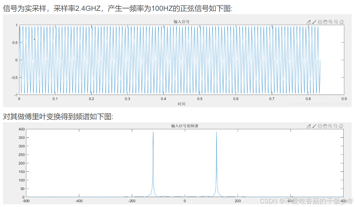
Signal_DDC = sin(2 * pi * 100 * Signal_DDC); % 生成一个频率为100Hz的正弦信号作为输入信号
- 这里定义了一个采样率为
FS的正弦信号,频率为 100 Hz。
2. 输入信号的时域和频域展示
N = length(Signal_DDC);
nfft = 2^nextpow2(N); % 计算合适的FFT长度
t_axis = (0:N-1) / FS; % 时间轴
f_axis = (0:nfft-1) / nfft * FS - FS / 2; % 频率轴

subplot(211)
plot(t_axis .* 1e6, real(Signal_DDC)); % 绘制输入信号的时域图
xlabel('时间 (\mu s)')
title('输入信号')

subplot(212)
Signal_DDC_fft = fftshift(fft(Signal_DDC, nfft)); % FFT变换并移频
plot(f_axis ./ 1e6, abs(Signal_DDC_fft)) % 绘制输入信号的频谱图
xlabel('频率 (MHz)')
title('输入信号的频谱')
- 使用
fftshift和fft函数计算并绘制信号的频谱图。
3. 多相滤波器组的设计与应用
fI = IF;
K = 32; % 子带数量
Channel_Freq_Range = [((0:K-1)-(K-1)/2).*FS/K-FS/K/2; ((0:K-1)-(K-1)/2).*FS/K+FS/K/2] ./ 1e6; % 每个子带的频率范围

h_LP = fir1(1023, 1/K, 'low'); % 设计低通滤波器
M = length(h_LP);
Q = fix(M / K);
H = zeros(K, Q);
for d = 1:K
    H(d, :) = h_LP(d:K:(Q-1)*K+d); % 将滤波器系数分解为多相分量
end
- 定义了
K=32个子带,并设计了一个低通滤波器。 - 将滤波器系数分解为多相分量,以便于后续的多相滤波器组实现。
4. 多相滤波器组的实现
tic;
temp = mod(length(Signal_DDC), K);
if temp ~= 0
    Signal_DDC0 = [Signal_DDC(1:end), zeros(1, K-temp)];
else
    Signal_DDC0 = Signal_DDC(1:end);
end
X = reshape(Signal_DDC0, K, length(Signal_DDC0) / K); % 重排信号为K行矩阵
X = flipud(X); % 翻转矩阵

[rx, L] = size(X);
if mod(K, 2) == 0
    X = X .* repmat((-1).^(0:L-1), K, 1); % 对偶数子带进行符号调整
end

Y = zeros(K, L);
for d = 1:K
    Y(d, :) = Filter_FFT(X(d, :), H(d, :)); % 对每个子带进行滤波
end

for ll = 1:L
    temp = Y(:, ll) .* (-1).^(0:K-1)';
    temp = temp .* exp(j * (0:K-1)' * pi / K);
    Y(:, ll) = ifft(temp, K) .* K; % IFFT变换并调整幅度
end
toc;
- 将输入信号重排为
K行矩阵,并根据子带数量进行必要的零填充。 - 对每个子带进行滤波和IFFT变换,得到每个子带的输出。
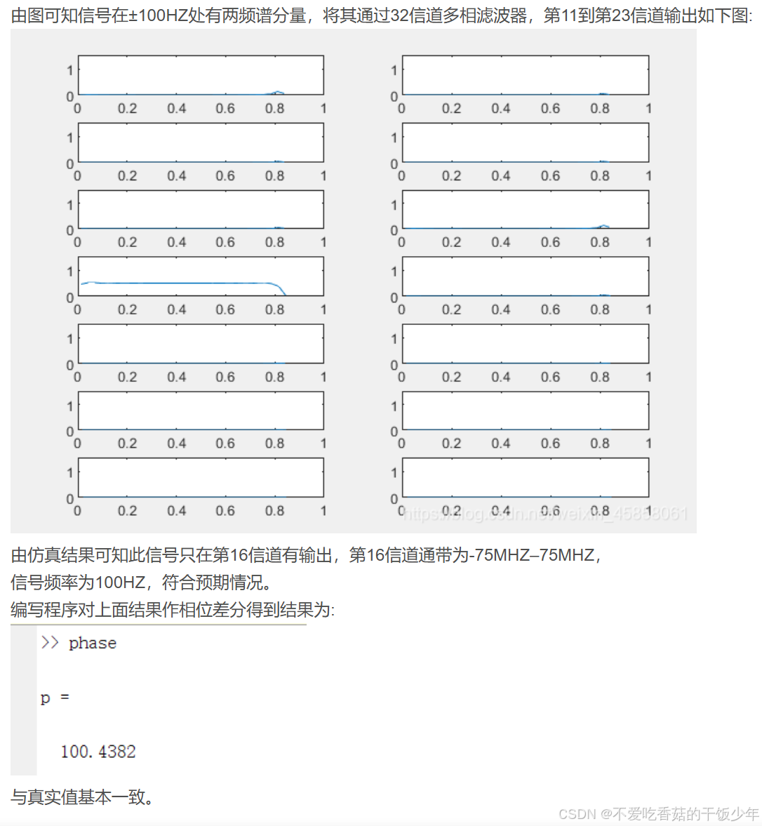
5. 子带信号的时间域展示
figure;
range = 14:27;
for d = 1:length(range)
    if mod(length(range), 2) == 0
        subplot(length(range) / 2, 2, d);
    else
        subplot((length(range) + 1) / 2, 2, d);
    end
    t_axis = ((0:L-1)) ./ FS .* K + (range(d)-1) ./ FS;
    plot(t_axis .* 1e6, abs(Y(range(d), :)));
    ylim([0 max(max(abs(Y))) + 1]);
end
- 绘制选定子带(
range = 14:27)的时域图。
6. 频率估计
for m = 1:460
    f = 150 + m * 5; % 生成不同频率的信号
    sig = floor(127 * sin(2 * pi * f * t));

    sig_vec = reshape(sig, 32, N / 32)';
    y = fft(sig_vec, [], 2);
    y = y(:, 1:16);

    [max_value, max_idx] = max(abs(y(1, :)));
    phase_ori = angle(y(:, max_idx))';

    sub_pse_ori = phase_ori(1, 2:end) - phase_ori(1, 1:end-1);
    for n = 1:length(sub_pse_ori)
        if (sub_pse_ori(1, n) >= pi)
            sub_pse_hand(1, n) = sub_pse_ori(1, n) - 2 * pi;
        elseif (sub_pse_ori(1, n) <= -pi)
            sub_pse_hand(1, n) = sub_pse_ori(1, n) + 2 * pi;
        else
            sub_pse_hand(1, n) = sub_pse_ori(1, n);
        end
    end

    pse_unwrap = unwrap(phase_ori);
    sub_pse_unwrap = pse_unwrap(1, 2:end) - pse_unwrap(1, 1:end-1);
    diff = sub_pse_hand - sub_pse_unwrap;

    sub_pse_0 = sub_pse_hand;
    ratio_0 = sum(sub_pse_0(1, 1:8)) / 8 / 2 / pi;
    sub_pse_1 = sub_pse_unwrap;
    ratio_1 = sum(sub_pse_1(1, 1:8)) / 8 / 2 / pi;
    a_result(1, m) = max_idx - 1 + ratio_0;
    b_result(1, m) = max_idx - 1 + ratio_1;
    c_result(1, m) = f / FS * 32;
end
- 生成一系列不同频率的信号,并对这些信号进行FFT变换。
- 计算每个信号的最大频率索引及其相位信息,并进行相位解缠绕。
- 根据相位差值估算频率,并将结果存储在
a_result和b_result中。
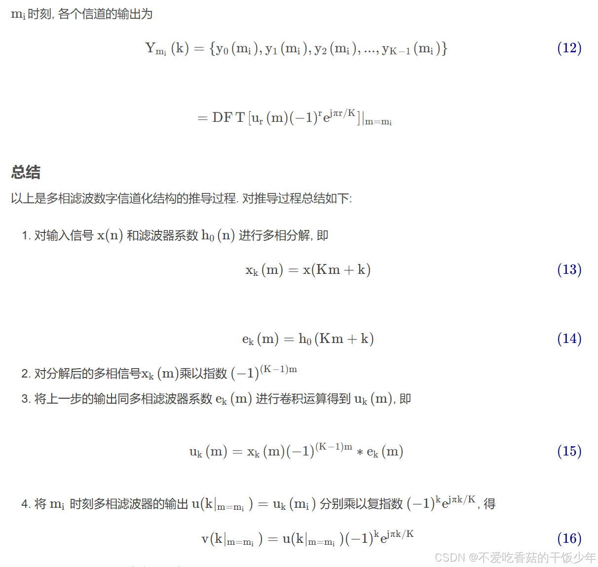
总结
这段代码的主要目的是:
- 生成和展示一个简单的正弦信号:通过时域和频域展示该信号。
- 实现一个多相滤波器组:用于将信号分成多个子带,并对每个子带进行滤波和处理。
- 频率估计:通过对不同频率信号的相位信息进行分析,估计其频率。
需要注意的是,代码中有一些未定义的函数(如 Filter_FFT),这可能是自定义函数或库函数。如果需要完整运行此代码,需确保所有函数都已定义或导入。此外,代码中的一些变量和逻辑可能需要根据具体需求进一步调整和优化。
clear all;close all;clc;
figure;
FS=2.4e+9;
IF=35e+7;
MF=3.6e+9;
Signal_DDC=0:1:1000;
Signal_DDC=Signal_DDC/1000;
Signal_DDC=sin(2*pi*100*Signal_DDC);


N=length(Signal_DDC);
nfft=2^nextpow2(N);
t_axis=(0:N-1)./fs;
f_axis=(0:nfft-1)./nfft*fs-fs/2;
subplot(211)
plot(t_axis.*1e6,real(Signal_DDC));
xlabel('时间')
title('输入信号')
subplot(212)
Signal_DDC_fft=(fftshift(fft(Signal_DDC,nfft)));
plot(f_axis./1e6,(abs(Signal_DDC_fft)))
xlabel('频率')
title('输入信号的频谱')

fI=IF;
K=32;
Channel_Freq_Range=[((0:K-1)-(K-1)/2).*fs/K-fs/K/2;((0:K-1)-(K-1)/2).*fs/K+fs/K/2]./1e6;

h_LP=fir1(1023,1/K,'low');
M=length(h_LP);
Q=fix(M/K);
H=zeros(K,Q);
for d=1:K
    H(d,:)=h_LP(d:K:(Q-1)*K+d);
end

tic;
temp=mod(length(Signal_DDC),K);
if temp~=0
    Signal_DDC0=[Signal_DDC(1:end),zeros(1,K-temp)];
    X=reshape(Signal_DDC0,K,length(Signal_DDC0)/K);
else
    X=reshape(Signal_DDC(1:end),K,length(Signal_DDC)/K);
end
X=flipud(X);

[rx,L]=size(X);
if mod(K,2)==0
    X=X.*repmat((-1).^(0:L-1),K,1);
end

Y=zeros(K,L);
for d=1:K
    Y(d,:)=Filter_FFT(X(d,:),H(d,:));
end
for ll=1:L
    temp=Y(:,ll).*(-1).^(0:K-1).';
    temp=temp.*exp(j*(0:K-1).'*pi/K);
    Y(:,ll)=ifft(temp,K).*K;
end
toc;

figure;
range=14:27;
for d=1:length(range)
    if mod(length(range),2)==0
        subplot(length(range)/2,2,d);
    else
        subplot((length(range)+1)/2,2,d);
    end
    t_axis=((0:L-1))./fs.*K+(range(d)-1)./fs;
    plot(t_axis.*1e6,abs(Y(range(d),:)))
    ylim([0 max(max(abs(Y)))+1])
End
for m=1:460
    f       = 150+m*5;
    sig     = floor(127*sin(2*pi*f*t));

    sig_vec = reshape(sig,32,N/32)';
    y       = fft(sig_vec,[],2);
    y       = y(:,1:16);


    [max_value,max_idx] = max(abs(y(1,:)));
    phase_ori = angle(y(:,max_idx))';


    sub_pse_ori = phase_ori(1,2:end) - phase_ori(1,1:end-1);
    for n = 1:length(sub_pse_ori)
       if(sub_pse_ori(1,n)>=pi)
           sub_pse_hand(1,n) = sub_pse_ori(1,n)-2*pi;
       elseif(sub_pse_ori(1,n)<=-pi)
           sub_pse_hand(1,n) = sub_pse_ori(1,n)+2*pi;
       else
           sub_pse_hand(1,n) = sub_pse_ori(1,n);
       end
    end

    pse_unwrap     = unwrap(phase_ori);
    sub_pse_unwrap = pse_unwrap(1,2:end) - pse_unwrap(1,1:end-1);
    diff = sub_pse_hand-sub_pse_unwrap;


    sub_pse_0 = sub_pse_hand;
    ratio_0 = sum(sub_pse_0(1,1:8))/8/2/pi;
    sub_pse_1 = sub_pse_unwrap;
    ratio_1 = sum(sub_pse_1(1,1:8))/8/2/pi;
    a_result(1,m) = max_idx-1+ratio_0;
    b_result(1,m) = max_idx-1+ratio_1;
    c_result(1,m) = f/FS*32;
end
转载于
设计32信道的多相滤波结构数字接收机
基于多相滤波器的数字信道化算法详解
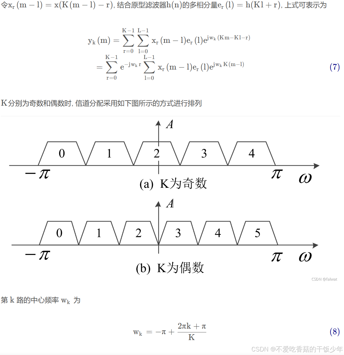
一 、实验题目
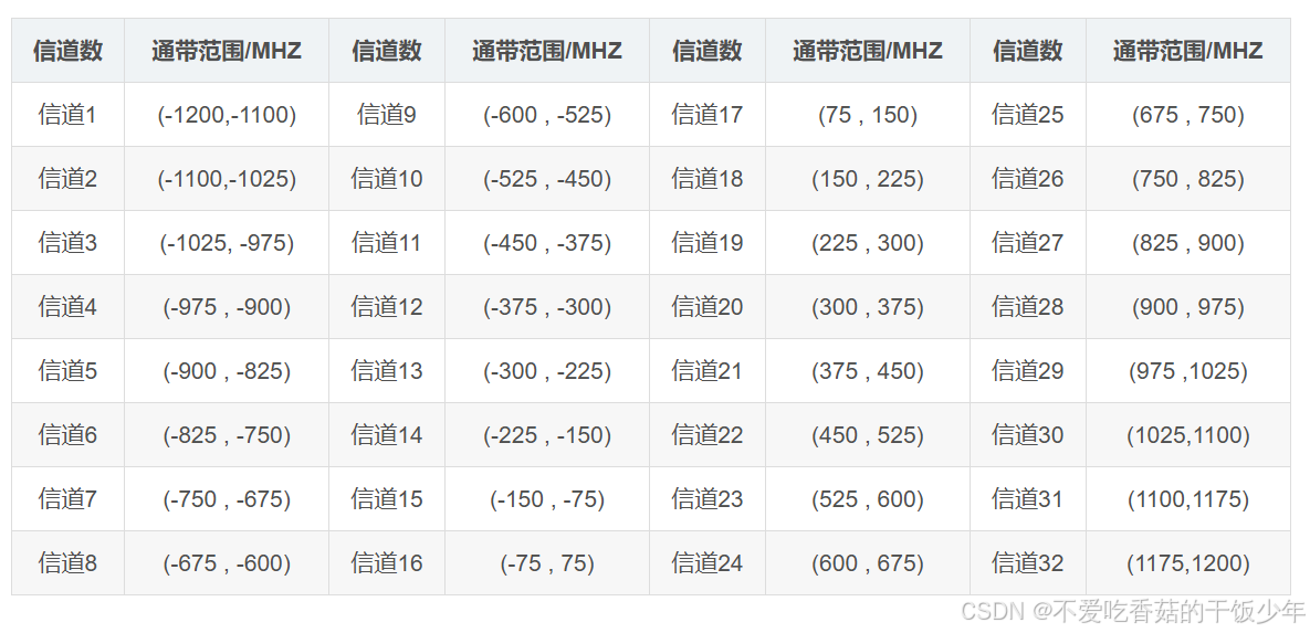
单通道实采样,采样率2.4GHz。设计32信道的多相滤波结构数字接收机,给出各信道的通带范围,采用MATLAB工具设计原型滤波器,给出原型滤波器特性。结合相位差分测频算法,输入不同频率的信号,测试数字接收机各信道输出,并完成信号频率测量。
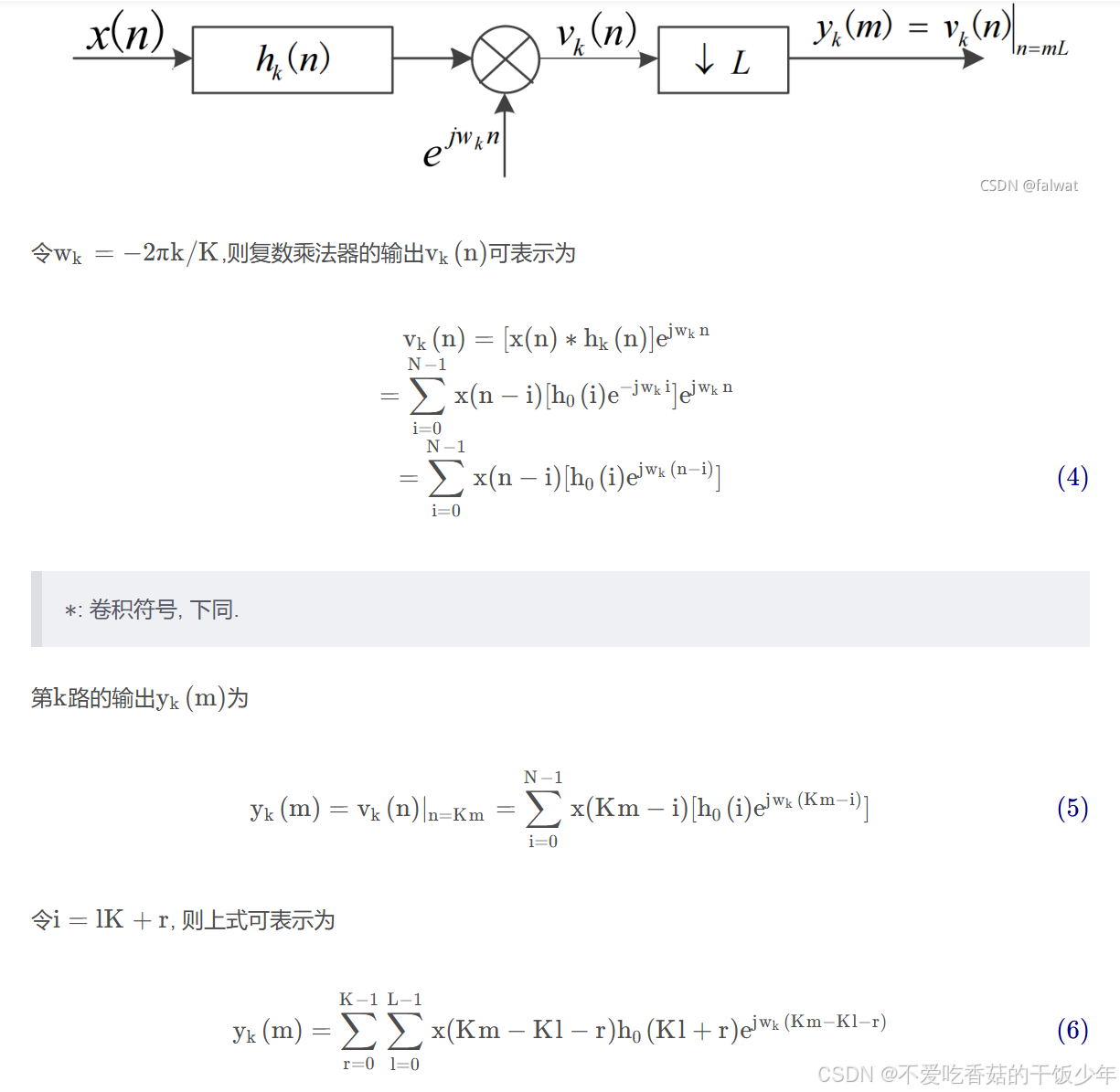
二、 实验原理
32信道多相滤波器结构图如下:

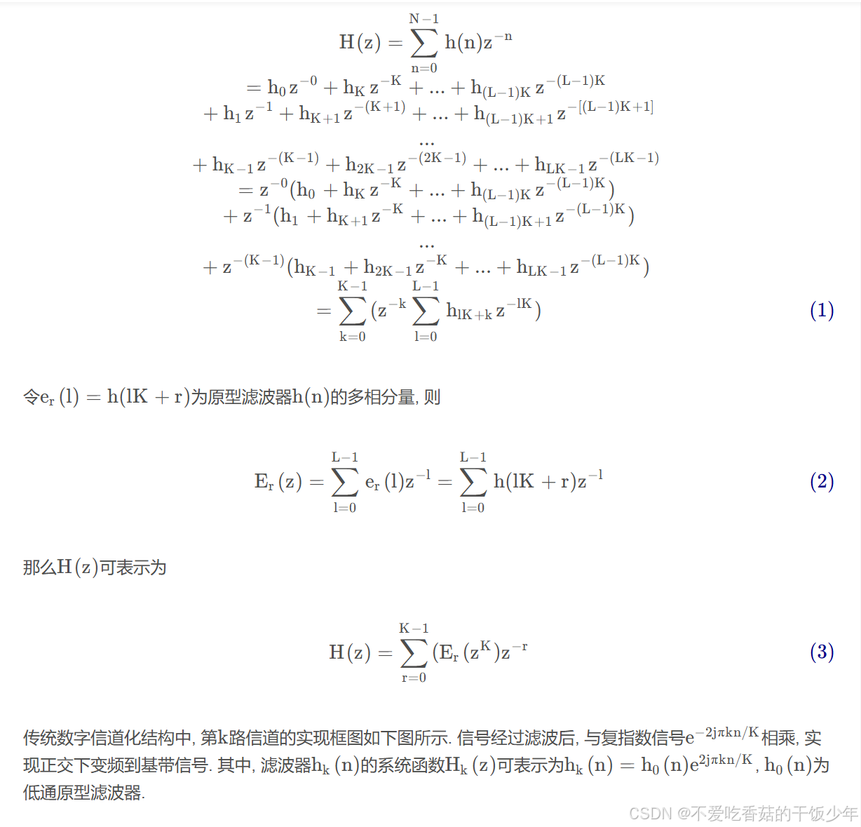
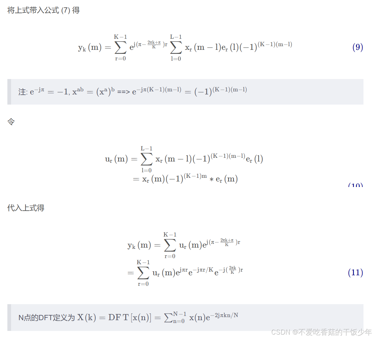
推导过程
多相滤波信道化是对传统信道化结构的改进, 通过各支路共用一个低通滤波器提高资源的利用率, 同时采用多相抽取提高了后续滤波和 FFT 的运算效率. 给定输入信号为x(n), 欲划分的信道数为K, 原型滤波器h(n)
的阶数为N NN, 且滤波器阶数能被信道数整除, 即L=N/K, 则原型滤波器的系统函数H(z)可表示为:

python仿真多相滤波器数字信道化算法
from scipy.signal import chirp, remez
import matplotlib.pyplot as plt
# [how to install `polyphase`](https://github.com/falwat/polyphase)
from polyphase import Channelizer
from numpy import arange, real, imag
from numpy.fft import fft, fftshift

 # 通道数
channel_num = 8
# 采样率
fs = 1280000

f0 = 0
f1 = fs/2
t1 = 1


#
T = 1

t = arange(0, int(T*fs)) / fs

# 生成一个chirp信号
s = chirp(t, f0, t1, f1)

# 创建原型滤波器
cutoff = fs / channel_num / 2    # Desired cutoff frequency, Hz
trans_width = cutoff / 10  # Width of transition from pass band to stop band, Hz
numtaps = 128      # Size of the FIR filter.
taps = remez(numtaps, [0, cutoff - trans_width, cutoff + trans_width, 0.5*fs],
                    [1, 0], Hz=fs)

# 创建信道化器
channelizer = Channelizer(taps, channel_num)

ss = channelizer.dispatch(s)


segs = 500;
ns = int(fs/segs);
nss = int(ss.shape[1]/segs);


# 分段绘图
fig, axs = plt.subplots(3, 1)

for i in range(segs):
    s0 = s[i*ns:i*ns+ns]
    h0 = abs(fft(s0))
    ss0 = ss[0:4, i*nss:i*nss+nss]
    hh0 = abs(fftshift(fft(ss0)))
    for ax in axs:
        ax.cla()
    axs[0].set_title(r'original signal')
    axs[1].set_title(r'The spectrum of channelized signals')
    axs[2].set_title(r'Waveform of channelized signal(real part)')
    axs[0].plot(h0 / max(h0))
    axs[1].plot(abs(hh0.T / hh0.max()))
    axs[2].plot(real(ss0.T))
    plt.pause(0.05)
原文链接:https://blog.csdn.net/falwat/article/details/121595096
原文链接:https://blog.csdn.net/weixin_45858061/article/details/102986358


