【图像处理】利用numpy实现直方图均衡、自适应直方图均衡、对比度受限自适应直方图均衡

在这里插入图片描述
直方图均衡化是一种在图像处理技术，通过调整图像的直方图来增强图像的对比度。
本博客不利用opencv库，仅利用numpy、matplotlib来实现直方图均衡、自适应直方图均衡、对比度受限自适应直方图均衡

直方图均衡

包括四个流程

计算图像RGB三通道的归一化直方图
计算变换函数， $k$ 为输入像素值，输出像素值为 $s = T (k)$
$s=T(k)=(L-1)\sum_{j=0}^kp_r(r_j)=(L-1)\sum_{j=0}^k\frac{n_j}{MN}=\frac{L-1}{MN}\sum_{j=0}^kn_j$
其中L=256，表示256个像素值， $p_r(r_j)$ 表示像素值为 $j$ 的像素点概率，MN表示像素点个数， $n_j$ 表示像素值为j的像素点个数， $k\in[0, L-1]$
对于每个通道的每个像素点，通过变换函数实现变换
三个通道的所有像素点变换后，合并起来，组合成新的RGB图像
直方图均衡利用全图的直方图统计信息，提升全图的对比度，对局部图的对比度提升较小，所以需要自适应直方图均衡。

自适应直方图均衡（Adaptive Histogram Equalization, AHE）

包括4个步骤

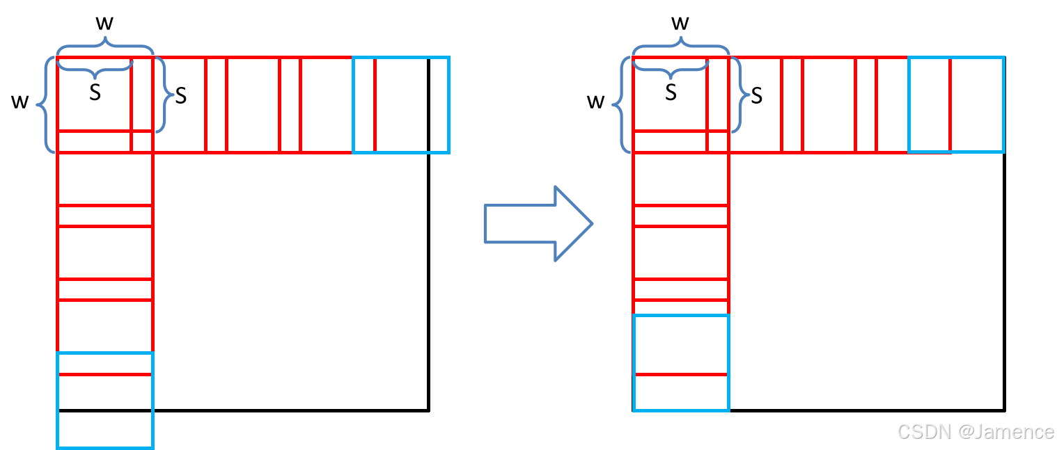
设置滑动窗口大小W (window size)以及步长S (stride)，需要保证W>=S
滑动窗口从图像左上角开始，向右、向下滑动。滑动过程中，窗口可能会滑出图像区域。为了避免该情况，如果窗口超出图像区域，把图像拉回来，贴到最近的边缘。如下图，蓝色窗口滑出图像区域，将其拉回。
对滑动窗口内的像素值统计直方图，进行变换。包括：
- 在窗口W*W区域内，统计直方图
- 在窗口W*W区域内，计算变换函数
- 如果窗口位于图像边缘（窗口在图像四个角、四条边上），变换函数作用于窗口内所有像素点
- 如果窗口位于图像内，变换函数仅作用于窗口中心的S*S区域，可以理解为利用窗口的统计信息优化窗口内局部区域的对比度
三个通道的所有像素点变换后，合并起来，组合成新的RGB图像
自适应直方图均衡对滑动窗口内的图像进行对比度增强，提升图像局部的对比度。一方面，局部对比度提升过大，容易失真；另一方面，不同局部区域的直方图统计信息差距明显，导致增强后的图像有明显的块状结构。

对比度受限自适应直方图均衡（Contrast Limited Adaptive histogram equalization, CLAHE）

具备6个步骤

设置滑动窗口W，直方图阈值T。
滑动窗口从图像左上角开始，向右、向下滑动。滑动过程中，窗口可能会滑出图像区域。为了避免该情况，采用和直方图均衡不同的策略，对原图做边缘的零填充。
对滑动窗口内的像素值进行变换。变换逻辑为：
- 在窗口W*W区域内，统计直方图
- 通过对直方图裁剪，限制对比度。将直方图中超过直方图阈值T的部分均分到直方图的每个块中。
- 计算每个窗口的变换函数
- 通过对目标窗口的像素值进行插值，缓解自适应直方图均衡带来的分块问题
  - 目标窗口D内，目标像素点位于4个子窗口，a、b、c、d
  - 每个子窗口有4个上、下、左、右的领域窗口。例如子窗口a的领域窗口是A、B、C、D，子窗口b的领域窗口是B、M、D、E。
  - 需要讨论一些边界情况：如果窗口D在图像的左上角，那么子窗口a的领域窗口只有D；如果窗口D在紧挨图像上边缘，那么子窗口b的领域窗口只有D和E…
  - 通过目标像素点和领域窗口的插值，实现变换。例如，对于在子窗口a的像素点，先计算在A、B、C、D四个窗口变换函数下的变换值，通过距离插值，得到最终变换值。
  - 三个通道的所有像素点变换后，合并起来，组合成新的RGB图像

实验对比结果

对于自适应直方图均衡，参数设置为：W=64, S=20
对于对比度受限自适应直方图均衡，参数设置为：W=40, T=10
ori：原图
1：直方图均衡
2：自适应直方图均衡
3：对比度受限自适应直方图均衡

样例1

在这里插入图片描述
RGB三通道直方图比较：

样例2

在这里插入图片描述
RGB三通道直方图比较：

三种算法比较

	直方图均衡	自适应直方图均衡	对比度受限自适应直方图均衡
增强效果	对比度较原图增强；图像较连续；局部区域增强不明显，部分局部区域比较暗	对比度较原图增强；图像不连续，有块状效应；局部区域增强较明显	对比度较原图增强；图像连续，无块状效应；局部区域对比度也有提升
直方图比较	直方图变得均衡，但首或尾可能值特别大	直方图变得均衡，但首或尾值依旧比其他位置大	直方图均衡化程度没有前两者高
运行时间	快	慢	中等

整体代码

import matplotlib.pyplot as plot
import PIL
import numpy as np
from pylab import    subplots_adjust
depth = 3

def show_histogram(img):
    """
    展示三个通道直方图

    :param img: 图像（numpy）
    :return: void，但是显示图像
    """
    plot.subplot(3, 1, 1)
    plot.hist(img[:, :, 0].flatten(), 256)
    plot.subplot(3, 1, 2)
    plot.hist(img[:, :, 1].flatten(), 256)
    plot.subplot(3, 1, 3)
    plot.hist(img[:, :, 2].flatten(), 256)
    plot.show()

def get_histogram(img, normed = True) :
    """
    计算img的直方图

    由于img有三个通道，需要在三个通道上做直方图，根据norm参数设置为0~1的概率值还是整数值

    :param img: 三维矩阵，长*宽*通道数
    :param normd: 是否做归一化
    :return: 在rgb通道上的直方图
    """
    his = np.zeros((3, 256))
    total_num = img.shape[0] * img.shape[1]
    for dep in range(depth) :
        for hei in range(img.shape[0]) :
            for wid in range(img.shape[1]) :
                his[dep][img[hei][wid][dep]] += 1
    if normed == True :
        his /= total_num
    return his

def histogramEqualization(img, save_pth='no') :
    """
    计算直方图均衡化之后的图像

    计算+保存 直方图均衡化之后的图像

    :param img: 输入图像(numpy)
    :param save_pth: 保存路径
    :return:  直方图均衡之后的图像(numpy)
    """
    ### 计算直方图
    his = get_histogram(img, normed = True)
    ### 计算累加和
    his_culsum = np.zeros((3, 256))
    for dep in range(depth) :
        sum_tmp = 0.0
        for index in range(256) :
            sum_tmp += his[dep][index]
            his_culsum[dep][index] = sum_tmp

    his_cdf = 255.0 * his_culsum

    ### Q1  整数化处理(测试三种取整方式)？
    # his_cdf = np.around(his_cdf, 0)
    his_cdf = np.floor(his_cdf)
    # img_hisequa = np.zeros(img.shape)
    ### Q2  保存图片前后的直方图不同意？
    ### Q3  numpy类型图片颜色显示不正确？

    ### 设置映射
    new_photo = PIL.Image.new('RGB', (img.shape[1], img.shape[0]))
    img_hisequa = np.array(new_photo)
    for hei in range(img.shape[0]) :
        for wid in range(img.shape[1]) :
            r = img[hei][wid][0]
            g = img[hei][wid][1]
            b = img[hei][wid][2]
            img_hisequa[hei][wid][0] ,img_hisequa[hei][wid][1], img_hisequa[hei][wid][2] = int(his_cdf[0][r]),  int(his_cdf[1][g]),  int(his_cdf[2][b])
    if save_pth != 'no' :
        img = PIL.Image.fromarray(img_hisequa.astype('uint8')).convert('RGB')
        img.save(save_pth, quality= 95)
    return img_hisequa

def AHE(img, W, S, save_pth = 'no') :
    """
    对图像做自适应直方图均衡化

    对图像做自适应直方图均衡化，保存到save_pth(当save_pth=no时不处理)

    :param img: 输入numpy图像
    :param W: 窗口边长参数W
    :param S: 影响区域大小边长/stride
    :param save_pth: 保存图像路径
    :return:
    """
    assert W >= S
    ### 按照S得到在水平方向和竖直方向滑动的次数，如果不能取整，加一
    img_height = img.shape[0]
    img_width = img.shape[1]
    hei_num = img_height / S
    if hei_num > int(hei_num) :
        hei_num = int(hei_num) + 1
    else:
        hei_num = int(hei_num)

    wid_num = img_width / S
    if wid_num > int(wid_num) :
        wid_num = int(wid_num) + 1
    else :
        wid_num = int(wid_num)
    print(hei_num, wid_num)

    # 处理边缘（采用窗口为W，影响区域为W处理，最后一个区域采用同样的W大小，可以忽视重叠部分）
    new_photo = PIL.Image.new('RGB', (img_width, img_height))
    img_hisequa = np.array(new_photo)
    for hei_i in range(1, hei_num + 1) :
        sta_hei = S * (hei_i - 1)
        end_hei = S * (hei_i)
        if end_hei > img_height :
            sta_hei = img_height - W
            end_hei = img_height
        img_hisequa[sta_hei:end_hei, 0: W, :] = histogramEqualization(img[sta_hei:end_hei, 0: W, :])
        img_hisequa[sta_hei:end_hei, img_width - W: img_width, :] = histogramEqualization(img[sta_hei:end_hei, img_width - W: img_width, :])
    for wid_i in range(1, wid_num + 1) :
        sta_wid = S * (wid_i - 1)
        end_wid = S * (wid_i)
        if end_wid > img_width :
            sta_wid = img_width - W
            end_wid = img_width
        img_hisequa[0: W, sta_wid: end_wid, :] = histogramEqualization(img[0: W, sta_wid: end_wid, :])
        img_hisequa[img_height - W: img_height, sta_wid: end_wid, :] = histogramEqualization(img[img_height - W: img_height, sta_wid: end_wid, :])

    #其次处理内部
    ### 类似的，计算内部区域滑动次数，有小数，加一
    pad_num = int((W - S) / 2)
    assert (W - S) % 2 == 0
    img_height_inside = img_height - 2 * W
    img_width_inside = img_width - 2 * W
    hei_num_inside = img_height_inside / S
    if hei_num_inside > int(hei_num_inside) :
        hei_num_inside = int(hei_num_inside) + 1
    else :
        hei_num_inside = int(hei_num_inside)
    wid_num_inside = img_width_inside / S
    if wid_num_inside > int(wid_num_inside) :
        wid_num_inside = int(wid_num_inside) + 1
    else :
        wid_num_inside = int(wid_num_inside)
    ### 将窗口W按照S滑动，最后一个区域也采用W窗口，影响区域为S，尽管会重叠，但是效果相同
    base_left = W
    base_right = img_width - W
    base_up = W
    base_down = img_height - W
    for hei_i in range(1, hei_num_inside + 1) :
        for wid_i in range(1, wid_num_inside + 1) :
            up = base_up + S * (hei_i - 1)
            down = base_up + S * hei_i
            if down > base_down :
                up = base_down - S
                down = base_down
            left = base_left + S * (wid_i - 1)
            right = base_left + S * wid_i
            if right > base_right :
                left = base_right - S
                right = base_right
            img_tmp = histogramEqualization(img[up - pad_num: down + pad_num, left - pad_num: right + pad_num, :])
            img_hisequa[up: down, left: right, :] = img_tmp[pad_num: img_tmp.shape[0] - pad_num, pad_num: img_tmp.shape[1] - pad_num,:]
    if save_pth != 'no' :
        img_save = PIL.Image.fromarray(img_hisequa.astype('uint8')).convert('RGB')
        img_save.save(save_pth, quality = 95)
    return img_hisequa

def clip(his, threshold = 1.0) :
    """
    裁剪直方图，阈值threshold = threshold_value * len(his) / total_num


    :param his:  直方图numpy（一维）
    :param threshold: 阈值 threshold_value * len(his) / total_num，
            threshold_value表示数量
    :return:裁剪之后的直方图
    """
    total_num = np.sum(his)
    # print(total_num)
    threshold_value = total_num / len(his) * threshold
    value_average = 0
    for i in range(len(his)) :
        if his[i] >= threshold_value :
            value_average += his[i] - threshold_value
    value_average /= len(his)
    his_clip = np.zeros(his.shape)
    for i in range(len(his)) :
        if his[i] >= threshold_value :
            his_clip[i] = threshold_value + value_average
        else :
            his_clip[i] = his[i]  + value_average
    return his_clip

def get_his_clip_histogramEqualization(img, threshold = 1.0) :
    """
    对裁剪后的直方图做均衡，在单通道上实现，其中调用了clip函数。

    :param img: 输入图片（单通道图片numpy）
    :param threshold:阈值threshold = threshold_value * len(his) / total_num
    :return:返回直方图的累计分布函数（即映射函数）
    """
    his = np.zeros(256)
    total_num = img.shape[0] * img.shape[1]
    for hei in range(img.shape[0]):
        for wid in range(img.shape[1]):
            his[img[hei][wid]] += 1
    his /= total_num
    his_clip = clip(his, threshold= threshold)

    his_culsum = np.zeros(256)
    sum_tmp = 0
    for index in range(256):
        sum_tmp += his_clip[index]
        his_culsum[index] = sum_tmp
    his_cdf = 255.0 * his_culsum
    his_cdf = np.floor(his_cdf)
    return his_cdf


def CLAHE_single_channel(img, W, T):
    """
    对单通道图像做CLAHE处理，即直方图裁剪+插值，其中调用了get_his_clip_histogramEqualization来
        得到裁剪后的直方图

    :param img: input image
    :param W:   window size W*W
    :param T:   histogram threshold = threshold_value * len(his) / sum(hist)
    :return:    对单通道图像做了CLAHE处理之后的单通道图像（numpy）
    """
    ### clip
    img_height = img.shape[0]
    img_width = img.shape[1]
    W_hei_num = (img_height // W)
    W_wid_num = (img_width // W)
    img = np.pad(img, ((0,W - (img_height - W_hei_num * W)),(0,W - (img_width - W_wid_num * W))),'constant',constant_values= (0,0))

    W_hei_num = img.shape[0] // W
    W_wid_num = img.shape[1] // W
    res_img = np.zeros(img.shape)
    ### 对单通道做直方图均衡
    #### 对整除的部分做处理
    his_map = {}
    for w_hei_i in range(W_hei_num):
        for w_wid_i in range(W_wid_num):
            up = w_hei_i * W
            down = (w_hei_i + 1) * W
            left = w_wid_i * W
            right = (w_wid_i + 1) * W
            his_tmp = get_his_clip_histogramEqualization(img[up: down, left: right], T)
            his_map[(w_hei_i, w_wid_i)] = his_tmp

    ### 插值
    for i_h in range(W_hei_num * W):
        for i_w in range(W_wid_num * W):
            ### 计算左上角的块在W_hei_num，W_wid_num块中的横纵坐标
            ## 从0开始，向下取整
            left_up_h = int((i_h - W / 2) / W)
            left_up_w = int((i_w - W / 2) / W)
            ### 计算距离
            dis_x = i_h - left_up_h * W - W / 2
            dis_x /= W
            dis_y = i_w - left_up_w * W - W / 2
            dis_y /= W
            ### 左上角
            if left_up_h < 0 and left_up_w < 0:
                res_img[i_h][i_w] = his_map[(left_up_h + 1, left_up_w + 1)][img[i_h, i_w]]
            ### 右上角
            elif left_up_h < 0 and left_up_w >= W_hei_num - 1:
                res_img[i_h][i_w] = his_map[(left_up_h + 1, left_up_w)][img[i_h, i_w]]
            ### 右下角
            elif left_up_h >= W_hei_num - 1 and left_up_w >= W_hei_num - 1:
                res_img[i_h][i_w] = his_map[(left_up_h, left_up_w)][img[i_h, i_w]]
            ### 左下角
            elif left_up_h >= W_hei_num - 1 and left_up_w < 0:
                res_img[i_h][i_w] = his_map[(left_up_h, left_up_w + 1)][img[i_h, i_w]]
            ### 四个边界
            ## 上边
            elif left_up_h < 0 :
                left = his_map[(0, left_up_w)][img[i_h, i_w]]
                right = his_map[(0, left_up_w + 1)][img[i_h, i_w]]
                res_img[i_h][i_w] = (1 - dis_y) * left + dis_y * right
            ## 下边
            elif left_up_h >= W_hei_num - 1 :
                left = his_map[(W_hei_num - 1, left_up_w)][img[i_h, i_w]]
                right = his_map[(W_hei_num - 1, left_up_w + 1)][img[i_h, i_w]]
                res_img[i_h][i_w] = (1 - dis_y) * left + dis_y * right
            ## 左边
            elif left_up_w < 0 :
                up = his_map[(left_up_h, 0)][img[i_h, i_w]]
                down = his_map[(left_up_h + 1, 0)][img[i_h, i_w]]
                res_img[i_h][i_w] = (1 - dis_x) * up + dis_x * down
            ## 右边
            elif left_up_w >= W_wid_num - 1 :
                up = his_map[(left_up_h, W_wid_num - 1)][img[i_h, i_w]]
                down = his_map[(left_up_h + 1, W_wid_num - 1)][img[i_h, i_w]]
                res_img[i_h][i_w] = (1 - dis_x) * up + dis_x * down
            else :
                left_up = his_map[(left_up_h, left_up_w)][img[i_h][i_w]]
                left_down = his_map[(left_up_h + 1, left_up_w)][img[i_h][i_w]]
                right_up = his_map[(left_up_h, left_up_w + 1)][img[i_h][i_w]]
                right_down = his_map[(left_up_h + 1, left_up_w + 1)][img[i_h][i_w]]
                res_img[i_h][i_w] = (1 - dis_y) * ((1 - dis_x) * left_up + dis_x * left_down) + dis_y * ((1 - dis_x) * right_up + dis_x * right_down)

    return res_img[:img_height, :img_width]
    ### 处理右边+下边的边界部分

def CLAHE(img, W,  T, save_pth = 'no') :
    """
    :param img: input image
    :param W:   window size W*W
    :param T:   histogram threshold = threshold_value * len(his) / sum(hist)
    :return:
    """
    # save_pth = 'astro_result3.jpg'
    res_img = img.copy()
    res_img[: ,:, 0] = CLAHE_single_channel(img[:,:,0],W,  T)
    res_img[:, :, 1] = CLAHE_single_channel(img[:,:,1],W,  T)
    res_img[:, :, 2] = CLAHE_single_channel(img[:,:,2],W,  T)
    if save_pth != 'no' :
        img_save = PIL.Image.fromarray(res_img.astype('uint8')).convert('RGB')
        img_save.save(save_pth, quality=95)
    return res_img

### 以下三个函数为测试直方图均衡化，自适应直方图均衡化，限制对比度自适应直方图均衡化，简单调用
def callhistogramEqualization() :
    img1_path = './rock.jpg'
    img1 = PIL.Image.open(img1_path, 'r')
    img1_numpy = np.array(img1)
    histogramEqualization(img1_numpy, 'rock_result1.jpg')
    show_histogram(img1_numpy)

    img1res_path = 'rock_result1.jpg'
    img1res = PIL.Image.open(img1res_path, 'r')
    img1res_numpy = np.array(img1res)
    show_histogram(img1res_numpy)

def callAHE() :
    img1_path = './rock.jpg'
    img1 = PIL.Image.open(img1_path, 'r')
    img1_numpy = np.array(img1)
    AHE(img1_numpy, W=48, S=16, save_pth='rock_result2.jpg')
    show_histogram(img1_numpy)

    img1res_path = 'rock_result2.jpg'
    img1res = PIL.Image.open(img1res_path, 'r')
    img1res_numpy = np.array(img1res)
    show_histogram(img1res_numpy)

def callCLAHE() :
    img1_path = './rock.jpg'
    img1 = PIL.Image.open(img1_path, 'r')
    img1_numpy = np.array(img1)
    CLAHE(img1_numpy, W=40,  T = 10, save_pth='rock_result3.jpg')
    # CLAHE(img1_numpy, W=40, A=0, T=10, save_pth='astro_result3.jpg')
    show_histogram(img1_numpy)

    img1res_path = 'rock_result3.jpg'
    img1res = PIL.Image.open(img1res_path, 'r')
    img1res_numpy = np.array(img1res)
    show_histogram(img1res_numpy)

def getResult() :
    img1Pth = './astronaut.jpg'
    img1 = PIL.Image.open(img1Pth, 'r')
    img1_numpy = np.array(img1)
    img1_numpy_he = histogramEqualization(img1_numpy)
    img1_numpy_ahe = AHE(img1_numpy, W=64, S=20)
    img1_numpy_clahe = CLAHE(img1_numpy, W=40, T = 10)

    fg = plot.figure()
    # plot.subplots_adjust(wspace=0, hspace=0)
    ax1 = plot.subplot(221)
    ax1.set_title('origin')
    ax1.axis('off')
    ax1.imshow(img1_numpy)

    ax2 = plot.subplot(222)
    ax2.set_title(1)
    ax2.axis('off')
    ax2.imshow(img1_numpy_he)

    ax3 = plot.subplot(223)
    ax3.set_title(2)
    ax3.axis('off')
    ax3.imshow(img1_numpy_ahe)

    ax4 = plot.subplot(224)
    ax4.set_title(3)
    ax4.axis('off')
    ax4.imshow(img1_numpy_clahe)
    plot.tight_layout()
    plot.savefig('./result_1.jpg')
    plot.show()


    img2Pth = './rock.jpg'
    img2 = PIL.Image.open(img2Pth, 'r')
    img2_numpy = np.array(img2)
    img2_numpy_he = histogramEqualization(img2_numpy)
    img2_numpy_ahe = AHE(img2_numpy, W=64, S=20)
    img2_numpy_clahe = CLAHE(img2_numpy, W=40, T = 10)

    plot.figure()
    ax1 = plot.subplot(221)
    ax1.set_title('origin')
    ax1.axis('off')
    ax1.imshow(img2_numpy)

    ax2 = plot.subplot(222)
    ax2.set_title(1)
    ax2.axis('off')
    ax2.imshow(img2_numpy_he)

    ax3 = plot.subplot(223)
    ax3.set_title(2)
    ax3.axis('off')
    ax3.imshow(img2_numpy_ahe)

    ax4 = plot.subplot(224)
    ax4.set_title(3)
    ax4.axis('off')
    ax4.imshow(img2_numpy_clahe)
    plot.tight_layout()
    plot.savefig('./result_2.jpg')
    plot.show()
if __name__ == "__main__" :
    # callhistogramEqualization()
    # callAHE()
    # callCLAHE()
    # img1res_path = 'astor_official_result2.jpg'
    # img1res = PIL.Image.open(img1res_path, 'r')
    # img1res_numpy = np.array(img1res)
    # show_histogram(img1res_numpy)
    getResult()