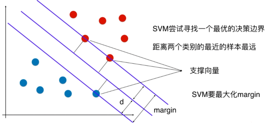
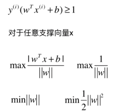
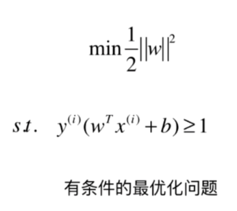
Support Vector Machine
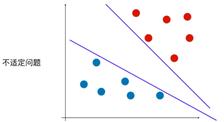
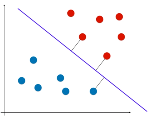
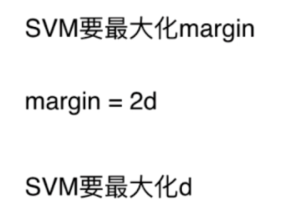
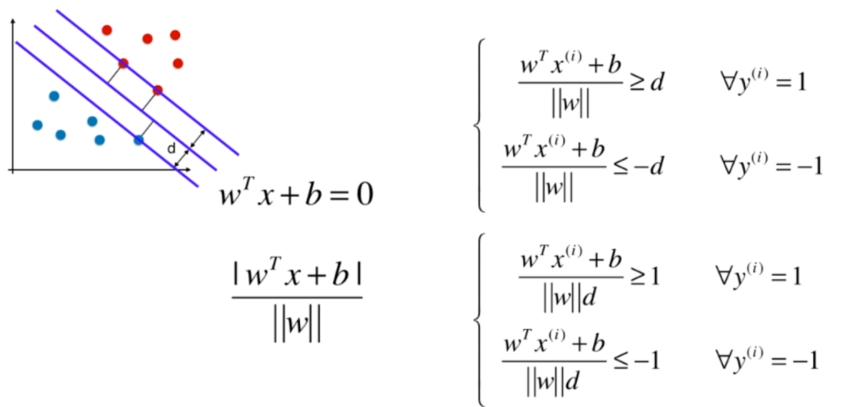
离分类样本尽可能远

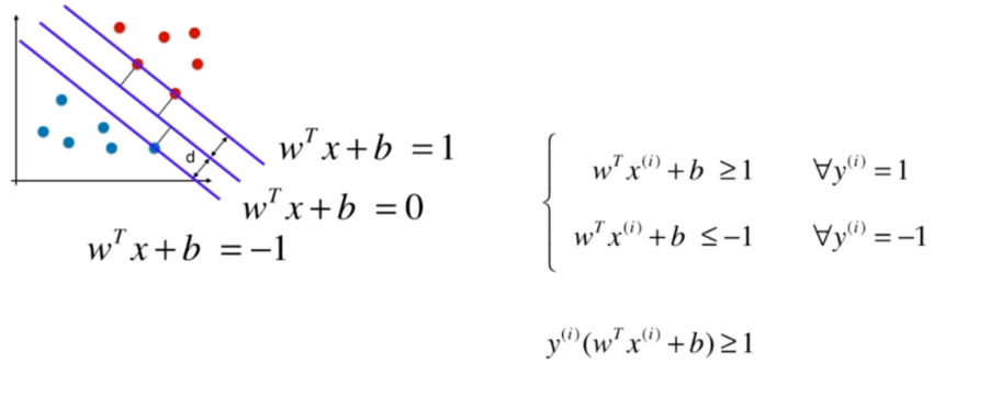
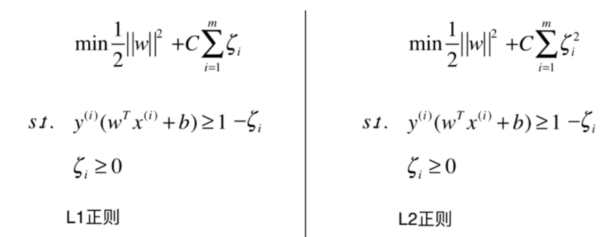
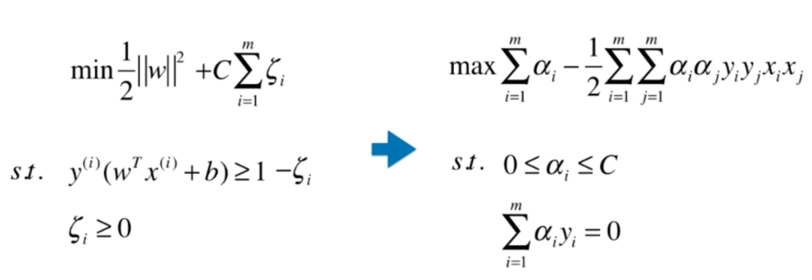
Soft Margin SVM
scikit-learn中的SVM
和kNN一样,要做数据标准化处理!
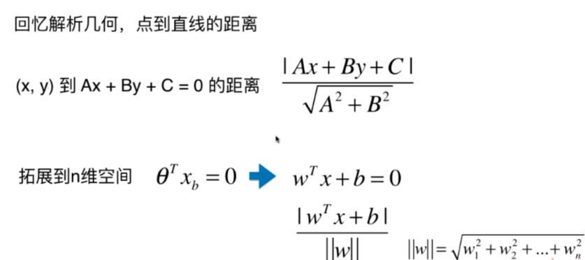
涉及距离!
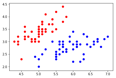
加载数据集
import numpy as np
import matplotlib.pyplot as plt
from sklearn import datasets

iris = datasets.load_iris()

X = iris.data
y = iris.target

X = X[y<2,:2]
y = y[y<2]
plt.scatter(X[y==0,0], X[y==0,1], color='red')
plt.scatter(X[y==1,0], X[y==1,1], color='blue')
plt.show()
数据标准化
from sklearn.preprocessing import StandardScaler

standardScaler = StandardScaler()
standardScaler.fit(X)
X_standard = standardScaler.transform(X)
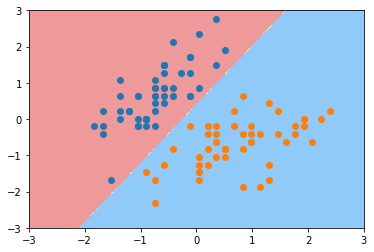
svm
from sklearn.svm import LinearSVC

svc = LinearSVC(C=1e9)
svc.fit(X_standard, y)
可视化
def plot_decision_boundary(model, axis):

    x0, x1 = np.meshgrid(
        np.linspace(axis[0], axis[1], int((axis[1]-axis[0])*100)).reshape(-1, 1),
        np.linspace(axis[2], axis[3], int((axis[3]-axis[2])*100)).reshape(-1, 1),
    )
    X_new = np.c_[x0.ravel(), x1.ravel()]

    y_predict = model.predict(X_new)
    zz = y_predict.reshape(x0.shape)

    from matplotlib.colors import ListedColormap
    custom_cmap = ListedColormap(['#EF9A9A','#FFF59D','#90CAF9'])

    plt.contourf(x0, x1, zz, linewidth=5, cmap=custom_cmap)
plot_decision_boundary(svc, axis=[-3, 3, -3, 3])
plt.scatter(X_standard[y==0,0], X_standard[y==0,1])
plt.scatter(X_standard[y==1,0], X_standard[y==1,1])
plt.show()
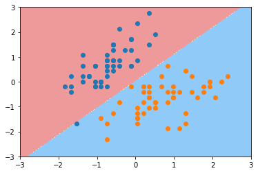
svc2 = LinearSVC(C=0.01)
svc2.fit(X_standard, y)
plot_decision_boundary(svc2, axis=[-3, 3, -3, 3])
plt.scatter(X_standard[y==0,0], X_standard[y==0,1])
plt.scatter(X_standard[y==1,0], X_standard[y==1,1])
plt.show()
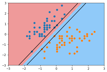
绘制上下对应的两条线
def plot_svc_decision_boundary(model, axis):

    x0, x1 = np.meshgrid(
        np.linspace(axis[0], axis[1], int((axis[1]-axis[0])*100)).reshape(-1, 1),
        np.linspace(axis[2], axis[3], int((axis[3]-axis[2])*100)).reshape(-1, 1),
    )
    X_new = np.c_[x0.ravel(), x1.ravel()]

    y_predict = model.predict(X_new)
    zz = y_predict.reshape(x0.shape)

    from matplotlib.colors import ListedColormap
    custom_cmap = ListedColormap(['#EF9A9A','#FFF59D','#90CAF9'])

    plt.contourf(x0, x1, zz, linewidth=5, cmap=custom_cmap)

    w = model.coef_[0]
    b = model.intercept_[0]

    # w0*x0 + w1*x1 + b = 0
    # => x1 = -w0/w1 * x0 - b/w1
    plot_x = np.linspace(axis[0], axis[1], 200)
    up_y = -w[0]/w[1] * plot_x - b/w[1] + 1/w[1]
    down_y = -w[0]/w[1] * plot_x - b/w[1] - 1/w[1]

    up_index = (up_y >= axis[2]) & (up_y <= axis[3])
    down_index = (down_y >= axis[2]) & (down_y <= axis[3])
    plt.plot(plot_x[up_index], up_y[up_index], color='black')
    plt.plot(plot_x[down_index], down_y[down_index], color='black')
plot_svc_decision_boundary(svc, axis=[-3, 3, -3, 3])
plt.scatter(X_standard[y==0,0], X_standard[y==0,1])
plt.scatter(X_standard[y==1,0], X_standard[y==1,1])
plt.show()
SVM中使用多项式特征
生成数据集
import numpy as np
import matplotlib.pyplot as plt
from sklearn import datasets

X, y = datasets.make_moons()
plt.scatter(X[y==0,0], X[y==0,1])
plt.scatter(X[y==1,0], X[y==1,1])
plt.show()
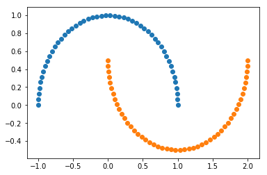
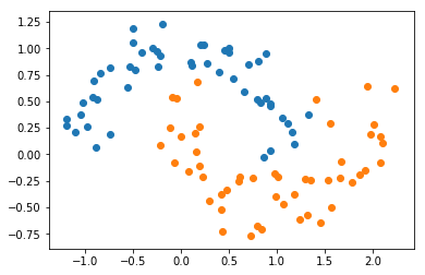
X, y = datasets.make_moons(noise=0.15, random_state=666)

plt.scatter(X[y==0,0], X[y==0,1])
plt.scatter(X[y==1,0], X[y==1,1])
plt.show()

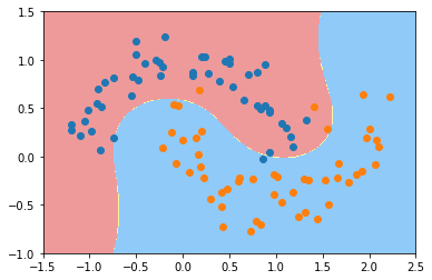
使用多项式特征的SVM
from sklearn.preprocessing import PolynomialFeatures, StandardScaler
from sklearn.svm import LinearSVC
from sklearn.pipeline import Pipeline

def PolynomialSVC(degree, C=1.0):
    return Pipeline([
        ("poly", PolynomialFeatures(degree=degree)),
        ("std_scaler", StandardScaler()),
        ("linearSVC", LinearSVC(C=C))
    ])
poly_svc = PolynomialSVC(degree=3)
poly_svc.fit(X, y)
def plot_decision_boundary(model, axis):

    x0, x1 = np.meshgrid(
        np.linspace(axis[0], axis[1], int((axis[1]-axis[0])*100)).reshape(-1, 1),
        np.linspace(axis[2], axis[3], int((axis[3]-axis[2])*100)).reshape(-1, 1),
    )
    X_new = np.c_[x0.ravel(), x1.ravel()]

    y_predict = model.predict(X_new)
    zz = y_predict.reshape(x0.shape)

    from matplotlib.colors import ListedColormap
    custom_cmap = ListedColormap(['#EF9A9A','#FFF59D','#90CAF9'])

    plt.contourf(x0, x1, zz, linewidth=5, cmap=custom_cmap)
plot_decision_boundary(poly_svc, axis=[-1.5, 2.5, -1.0, 1.5])
plt.scatter(X[y==0,0], X[y==0,1])
plt.scatter(X[y==1,0], X[y==1,1])
plt.show()
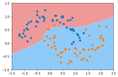
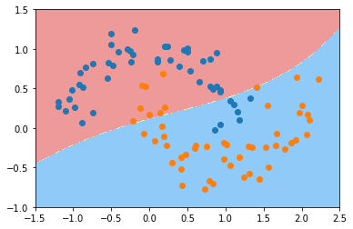
使用多项式核函数的SVM
from sklearn.svm import SVC

def PolynomialKernelSVC(degree, C=1.0):
    return Pipeline([
        ("std_scaler", StandardScaler()),
        ("kernelSVC", SVC(kernel="poly", degree=degree, C=C))
    ])
poly_kernel_svc = PolynomialKernelSVC(degree=3)
poly_kernel_svc.fit(X, y)
plot_decision_boundary(poly_kernel_svc, axis=[-1.5, 2.5, -1.0, 1.5])
plt.scatter(X[y==0,0], X[y==0,1])
plt.scatter(X[y==1,0], X[y==1,1])
plt.show()
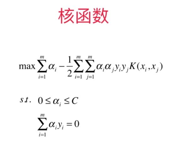
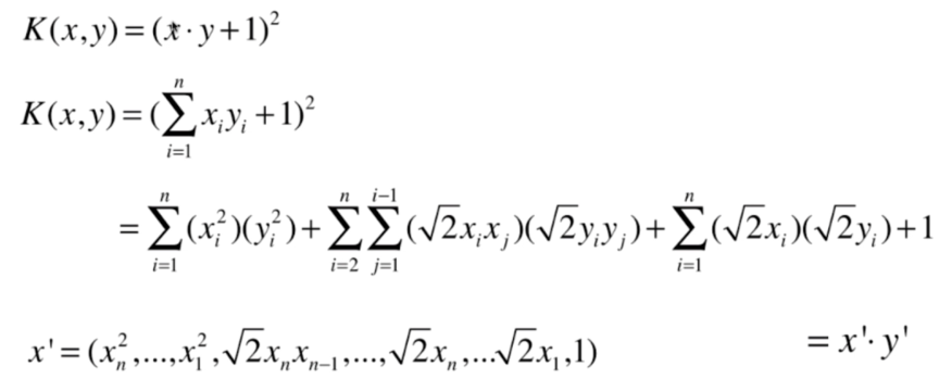
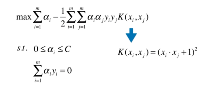
什么是核函数
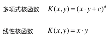
多项式核函数
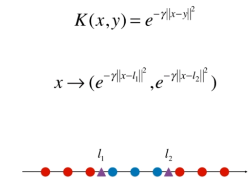
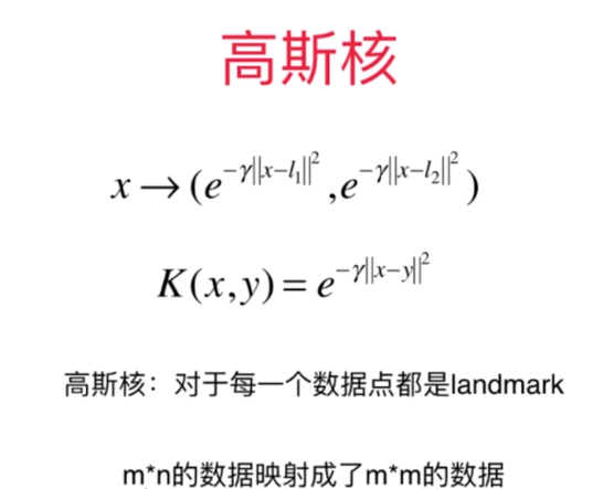
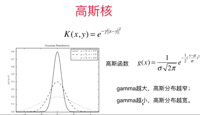
高斯核函数
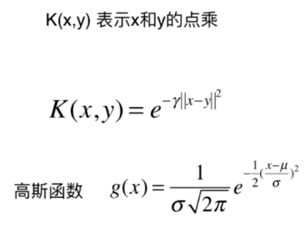
RBF核 Radial Basis Function Kernel
将每一个样本点映射到一个无穷维的特征空间
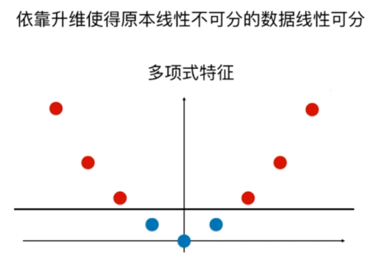
多项式特征
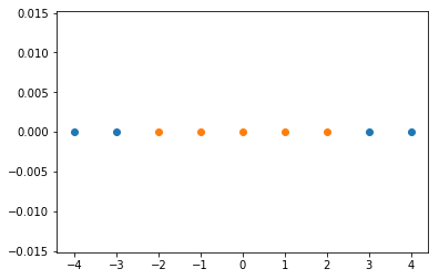
高斯核
import numpy as np
import matplotlib.pyplot as plt
x = np.arange(-4, 5, 1)
y = np.array((x >= -2) & (x <= 2), dtype='int')
plt.scatter(x[y==0], [0]*len(x[y==0]))
plt.scatter(x[y==1], [0]*len(x[y==1]))
plt.show()
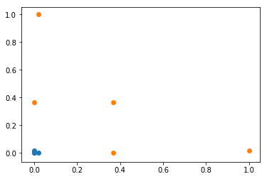
高斯核
def gaussian(x, l):
    gamma = 1.0
    return np.exp(-gamma * (x-l)**2)
l1, l2 = -1, 1

X_new = np.empty((len(x), 2))
for i, data in enumerate(x):
    X_new[i, 0] = gaussian(data, l1)
    X_new[i, 1] = gaussian(data, l2)
plt.scatter(X_new[y==0,0], X_new[y==0,1])
plt.scatter(X_new[y==1,0], X_new[y==1,1])
plt.show()
scikit-learn中的高斯核函数
import numpy as np
import matplotlib.pyplot as plt
from sklearn import datasets

X, y = datasets.make_moons(noise=0.15, random_state=666)

plt.scatter(X[y==0,0], X[y==0,1])
plt.scatter(X[y==1,0], X[y==1,1])
plt.show()
预处理
from sklearn.preprocessing import StandardScaler
from sklearn.pipeline import Pipeline
from sklearn.svm import SVC

def RBFKernelSVC(gamma):
    return Pipeline([
        ("std_scaler", StandardScaler()),
        ("svc", SVC(kernel="rbf", gamma=gamma))
    ])
svc = RBFKernelSVC(gamma=1)
svc.fit(X, y)
可视化
def plot_decision_boundary(model, axis):

    x0, x1 = np.meshgrid(
        np.linspace(axis[0], axis[1], int((axis[1]-axis[0])*100)).reshape(-1, 1),
        np.linspace(axis[2], axis[3], int((axis[3]-axis[2])*100)).reshape(-1, 1),
    )
    X_new = np.c_[x0.ravel(), x1.ravel()]

    y_predict = model.predict(X_new)
    zz = y_predict.reshape(x0.shape)

    from matplotlib.colors import ListedColormap
    custom_cmap = ListedColormap(['#EF9A9A','#FFF59D','#90CAF9'])

    plt.contourf(x0, x1, zz, linewidth=5, cmap=custom_cmap)
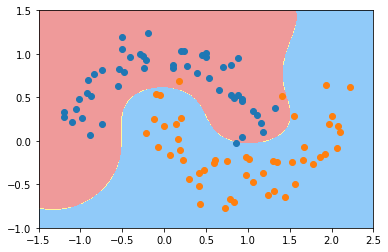
plot_decision_boundary(svc, axis=[-1.5, 2.5, -1.0, 1.5])
plt.scatter(X[y==0,0], X[y==0,1])
plt.scatter(X[y==1,0], X[y==1,1])
plt.show()
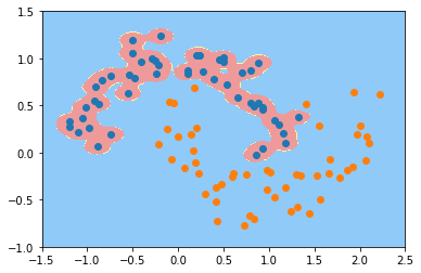
svc_gamma100 = RBFKernelSVC(gamma=100)
svc_gamma100.fit(X, y)
plot_decision_boundary(svc_gamma100, axis=[-1.5, 2.5, -1.0, 1.5])
plt.scatter(X[y==0,0], X[y==0,1])
plt.scatter(X[y==1,0], X[y==1,1])
plt.show()
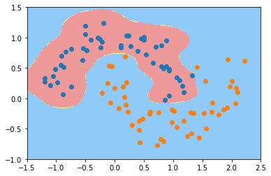
svc_gamma10 = RBFKernelSVC(gamma=10)
svc_gamma10.fit(X, y)
plot_decision_boundary(svc_gamma10, axis=[-1.5, 2.5, -1.0, 1.5])
plt.scatter(X[y==0,0], X[y==0,1])
plt.scatter(X[y==1,0], X[y==1,1])
plt.show()
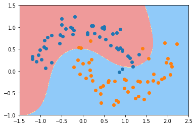
svc_gamma05 = RBFKernelSVC(gamma=0.5)
svc_gamma05.fit(X, y)
plot_decision_boundary(svc_gamma05, axis=[-1.5, 2.5, -1.0, 1.5])
plt.scatter(X[y==0,0], X[y==0,1])
plt.scatter(X[y==1,0], X[y==1,1])
plt.show()
svc_gamma01 = RBFKernelSVC(gamma=0.1)
svc_gamma01.fit(X, y)
plot_decision_boundary(svc_gamma01, axis=[-1.5, 2.5, -1.0, 1.5])
plt.scatter(X[y==0,0], X[y==0,1])
plt.scatter(X[y==1,0], X[y==1,1])
plt.show()
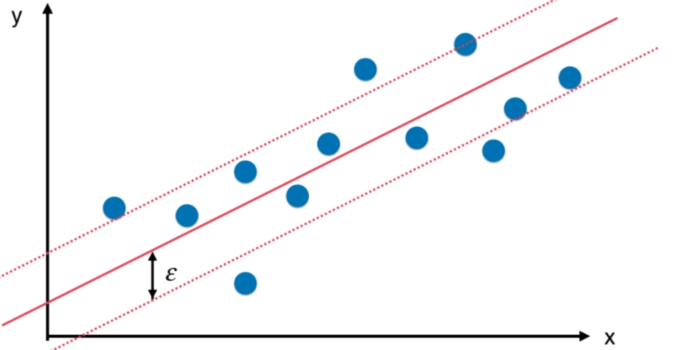
SVM思路解决回归问题
import numpy as np
import matplotlib.pyplot as plt
from sklearn import datasets

boston = datasets.load_boston()
X = boston.data
y = boston.target
from sklearn.model_selection import train_test_split

X_train, X_test, y_train, y_test = train_test_split(X, y, random_state=666)
from sklearn.svm import LinearSVR
from sklearn.svm import SVR
from sklearn.preprocessing import StandardScaler
from sklearn.pipeline import Pipeline

def StandardLinearSVR(epsilon=0.1):
    return Pipeline([
        ('std_scaler', StandardScaler()),
        ('linearSVR', LinearSVR(epsilon=epsilon))
    ])
svr = StandardLinearSVR()
svr.fit(X_train, y_train)
svr.score(X_test, y_test)