文章目录
- Graph Search Basis
- Configuration Space
- Configuration Space Obstacle
- Workspace and Configuration Space Obstacle
- Graph and Search Method
- Graph Search Overview
- Graph Traversal
- Breadth First Search (BFS)
- Depth First Search (DFS)
- versus
- Heuristic Search
- Greedy Best First Search
- Costs on Actions
- Dijkstra and A*
- Algorithm Workflow
- Dijkstra's Algorithm
- 伪代码
- Pros and Cons of Dijkstra's Algorithm
- Search Heuristics
- A*: Dijkstra with a Heuristic
- 伪代码
- A* Optimality
- Admissible Heuristics
- Heuristic Design
- Sub-optimal Solution
- Greedy Best First Search vs. Weighted A* vs. A*
- Engineering Considerations
- Grid-based Path Search
- Implementation
- The Best Heuristic
- Tie Breaker
- Jump Point Search
- Look Ahead Rule
- Jumping Rules
- pesudo-code
- Example
- Extension
- 3D JPS
- Is JPS always better?
- Homework
- Assignment: Basic
- Assignment: Advance
Graph Search Basis
Configuration Space
Robot degree of freedom (DOF): The minimum number n of real-valued coordinates need to represent the robot configuration.
Robot configuration space: a n-dim space containing all possible robot configurations, denoted as C-space
Each robot pose is a point in the C-space
Configuration Space Obstacle
Workspace - Configuration Space
- Obstacles need to be represented in configuration space (one-time work prior to motion planning), called configuration space obstacle, or C-obstacle.
- C-space = (C-obstacle) ∪ \cup ∪ (C-free)
- The path planning is finding a path between start
pointq s t a r t q_{start} qstart and goalpointq g o a l q_{goal} qgoal with C-free.
Workspace and Configuration Space Obstacle
- In workspace
Robot has shape and size - In configuration space: C-space
Robot isa point
Obstacle are represented in C-space prior to motion planning.
Graph and Search Method
Graphs: Graphs have nodes and edges
State space graph: a mathematical representation of a search algorithm.
Graph Search Overview
- Maintain a
containerto store all the nodesto be visited - The container is initialized with the start state X S X_S XS
- Loop
–Removea node from the container according to some pre-defined score function.
–Expansion: Obtain all neighbors of the node
–Pushthem (neighbors) into the container. - End Loop
Question 1: When to end the loop?
Possible option: End the loop when the container is empty.
Question 2: What if the graph is cyclic?
When a node is removed from the container (expand / visited), it should never be added back to the container again.
Question 3: In what way to remove the right node such that the goal state can be reached as soon as possible, which results in less expansion of the graph node.
Graph Traversal
Breadth First Search (BFS)
BFS uses “first in first out” = queue

- Strategy: remove / expand the shallowest node in the container
Depth First Search (DFS)
DFS uses “last in first out” = stack

- Strategy: remove / expand the deepest node in the container
- Implementation: maintain a last in first out (LIFO) container (i.e. stack)
versus

Breadth First Search(BFS,FIFO)能找出最短路径
Heuristic Search
Greedy Best First Search
-
BFS and DFS pick the next node off the frontiers based on which was “first in” or “last in”.
-
Greedy Best First picks the “best” node according to some rule, called a
heuristic. -
Definition: A heuristic is a
guessof how close you are to the target.

-
A heuristic guides you in the right direction.
-
A heuristic should be easy to compute.

Costs on Actions
- A practical search problem has a
cost "C"from a node to its neighbor- Length, time, energy, etc.
- When all weight are 1, BFS finds the optimal solution
- For general cases, how to find the
least-cost pathas soon as possible?
Dijkstra and A*
Algorithm Workflow
Dijkstra’s Algorithm
- Strategy: expand/visit the node with
cheapest accumulated cost g(n)- g(n): The current best estimates of the accumulated cost from the start state to node “n”
- Update the accumulated costs g(m) for all unexpected neighbors “m” of node “n”
- A node that has been expanded/visited is guaranteed to have the smallest cost from the start state.
伪代码
- Maintain a
priority queueto store all the nodes to be expanded - The priority queue is initialized with the start state X s X_s Xs
- Assign g ( X s ) = 0 g(X_s)=0 g(Xs)=0, and g(n)=infinite for all other nodes in the graph
- Loop
- If the queue is empty, return FALSE; break;
- Remove the node “n” with the lowest g(n) from the priority queue
- Mark node “n” as expanded
- If the node “n” is the goal state, return True; break;
- For all unexpanded neighbors “m” of node “n”
- If g(m) = infinite
- g(m) = g(n) + C n m C_{nm} Cnm
- Push node “m” into the queue
- If g(m) > g(n) +
C
n
m
C_{nm}
Cnm
- g(m) = g(n) + C n m C_{nm} Cnm
- If g(m) = infinite
- End
- End Loop
priority queue = container =
open list
已经扩展过的节点放到close list
Pros and Cons of Dijkstra’s Algorithm
- The good:
- Complete and optimal
- The bad:
- Can only see the accumulated so far (i.e. the uniform cost), thus exploring next state in every “direction”
- No information about goal location
Search Heuristics
- Recall the heuristic introduced in Greedy Best First Search
- Overcome the shortcomings of uniform cost search by
inferring the least cost to goal (i.e. goal cost) - Designed for particular search problem
- Examples: Manhattan distance VS. Euclidean distance
A*: Dijkstra with a Heuristic
- Accumulated cost
- g(n): The current best estimates of the accumulated cost from the start state to node “n”
- Heuristic
- h(n): The
estimated least costfrom node n to goal state (i.e. goal cost)
- h(n): The
- The least estimated cost from start node to goal state passing through node “n” is f(n)=g(n) + h(n)
- Strategy: expand the node with
cheapest f(n) = g(n )+ h(n)- Update the accumulated costs g(m) for all unexpanded neighbors “m” of node “n”
- A node that has been expanded is guaranteed to have the smallest cost from the start node
伪代码
- Maintain a
priority queueto store all the nodes to be expanded - The heuristic function h(n) for all nodes are pre-defined
- The priority queue is initialized with the start state X s X_s Xs
- Assign g ( X s ) = 0 g(X_s)=0 g(Xs)=0, and g(n)=infinite for all other nodes in the graph
- Loop
- If the queue is empty, return FALSE; break;
- Remove the node “n” with the lowest f(n) = g(n)+h(n) from the priority queue
- Mark node “n” as expanded
- If the node “n” is the goal state, return True; break;
- For all unexpanded neighbors “m” of node “n”
- If g(m) = infinite
- g(m) = g(n) + C n m C_{nm} Cnm
- Push node “m” into the queue
- If g(m) > g(n) +
C
n
m
C_{nm}
Cnm
- g(m) = g(n) + C n m C_{nm} Cnm
- If g(m) = infinite
- End
- End Loop
A* Optimality

- What went wrong?
- For node A: actual least cost to goal (i.e. goal cost) < estimated least cost to goal (i.e. heuristic)
- We need the estimate to be
less thanactual least cost to goal (i.e. goal cost)for all nodes!
Admissible Heuristics
- A Heuristic h is
admissible(optimistic) if:h(n) <= h*(n) forall node “n”, where h*(n) is the true least cost to goal from node “n”
- If the heuristic is admissible, the A* search is optimal
- Coming up with admissible heuristics is most of what’s involved in using A* in practice.
Heuristic Design
An admissible heuristic function has to be designed case by case.
-
Euclidean Distance
Is Euclidean distance (L2 norm) admissible?Always -
Manhattan Distance
Is Manhattan distance (L1 norm) admissible?Depends
Is L
∞
\infty
∞ norm distance admissible? Always
Is 0 distance admissible? Always
A* expands mainly towards the goal, but does not hedge its bets to ensure optimality.
Sub-optimal Solution
What if we intend to use an over-estimate heuristic?
Suboptimal path and Faster
Weighted A*: Expands states based on
f
=
g
+
ε
h
f = g + \varepsilon h
f=g+εh,
ε
>
1
\varepsilon>1
ε>1=bias towards states that are closer to goal.
- Weighted A* Search
- Optimality vs. speed
- ε \varepsilon ε-suboptimal: cost(solution) <= ε c o s t ( o p t i m a l s o l u t i o n ) \varepsilon cost(optimal solution) εcost(optimalsolution)
- It can be orders of magnitude faster than A*
Weighted A* -> Anytime A* -> ARA* -> D*
Greedy Best First Search vs. Weighted A* vs. A*

Engineering Considerations
Grid-based Path Search
- How to represent grids as graphs?
Each cell is a node. Edges connect adjacent cells.
Implementation
- Create a dense graph.
- Link the occupancy status stored in the grid map.
- Neighbors discovered by grid index.
- Perform A* search.
\;
- Priority queue in C++
- std::priority_queue
- std::make_heap
- std::multimap
The Best Heuristic
They are useful, but none of them is the best choice, why?
Because none of them is tight
Tight means who close they measure the true shortest distance.
Why so many nodes expanded?
Because Euclidean distance is far from the truly theoretical optimal solution.
\;
How to get the truly theoretical optimal solution
Fortunately, the grid map is highly structural.

- You don’t need to search the path.
- It has the
closed-form solution!
d x = a b s ( n o d e . x − g o a l . x ) d y = a b s ( n o d e . y − g o a l . y ) h = ( d x + d y ) + ( 2 − 2 ) ∗ m i n ( d x , d y ) dx = abs(node.x - goal.x)\\ dy = abs(node.y - goal.y)\\ h = (dx+dy) + (\sqrt2 - 2)*min(dx, dy) dx=abs(node.x−goal.x)dy=abs(node.y−goal.y)h=(dx+dy)+(2−2)∗min(dx,dy)
diagonal Heuristic
h(n) = h*(n)
Tie Breaker
-
Many paths have the same f value.
-
No differences among them making them explored by A* equally.

-
Manipulate the f f f value breaks tie
-
Make same f f f values differ.
-
Interfere h h h slightly.
- h = h × ( 1.0 + p ) h = h \times (1.0 + p) h=h×(1.0+p)
- p < m i n i m u m c o s t o f o n e s t e p e x p e c t e d m a x i m u m p a t h c o s t p < \frac{minimum \; cost \; of \; one \; step}{expected \; maximum \; path \; cost} p<expectedmaximumpathcostminimumcostofonestep
Core idea of tie breaker:
Find a preference among same cost paths
-
When nodes having same f f f, compare their h h h
-
Add deterministic random numbers to the heuristic or edge costs (A hash of the coordinates).
-
Prefer paths that are along the straight line from the starting point to the goal.
d x 1 = a b s ( n o d e . x − g o a l . x ) d y 1 = a b s ( n o d e . y − g o a l . y ) d x 2 = a b s ( s t a r t . x − g o a l . x ) d y 2 = a b s ( s t a r t . y − g o a l . y ) c r o s s = a b s ( d x 1 × d y 2 − d x 2 × d y 1 ) h = h + c r o s s × 0.001 dx1=abs(node.x - goal.x)\\ dy1 = abs(node.y - goal.y)\\ dx2 = abs(start.x - goal.x)\\ dy2 = abs(start.y - goal.y)\\ cross = abs(dx1\times dy2 - dx2\times dy1)\\ h = h+cross\times 0.001 dx1=abs(node.x−goal.x)dy1=abs(node.y−goal.y)dx2=abs(start.x−goal.x)dy2=abs(start.y−goal.y)cross=abs(dx1×dy2−dx2×dy1)h=h+cross×0.001 -
… Many customized ways
\;
- Prefer paths that are along the straight line from the starting point to the goal.

Jump Point Search
Core idea of JPS
Find symmetry and break them.

JPS explores intelligently, because it always looks ahead based on a rule.
Look Ahead Rule
Consider
- current node x x x
-
x
x
x’s expanded direction

Neighbor Pruning
- Gray nodes:
inferior neighbors, when going to them, the path without x x x is cheaper. Discard. - White nodes:
natural neighbors - We only need to consider natural neighbors when expand the search.

Forced Neighbors
- There is obstacle adjacent to x x x
- Red nodes are
forced neighbors. - A cheaper path from x x x’s parent to them is blocked by obstacle.
Jumping Rules

- Recursively apply
straightpruning rule and identify y as ajump point successorof x x x. This node is interesting because it has a neighbor z that cannot be reached optimally except by a path that visit x x x then y y y. - Recursively apply the
diagnol pruningrule and identify y as ajump point successorof x x x - Before each diagonal step we first recurse straight. Only if both straight recursions fail to identify a jump point do we step diagnally again.
- Node w, a forced neighbor of
x
x
x, is expanded as normal. (also push into the open list, the
priority queue)
pruning rule = look ahead rule
pesudo-code
Recall A* 's pseudo-code, JPS’s is all the same!
- Maintain a priority queue to store all the nodes to be expanded
- The heuristic function h(n) for all nodes are pre-defined
- The priority queue is initialized with the start state X s X_s Xs
- Assign g ( X s ) = 0 g(X_s)=0 g(Xs)=0, and g(n)=infinite for all other nodes in the graph
- Loop
- If the queue is empty, return FALSE; break;
Removethe node “n” with the lowest f(n) = g(n) + h(n) from the priority queue- Mark node “n” as
expanded - If the node “n” is the goal state, return TRUE, break;
- For all
unexpanded neighbors“m” of node “n”- If g(m) = infinite
- g(m) = g(n) + C n m C_{nm} Cnm
- Push node “m” into the queue
- If g(m) > g(n) +
C
n
m
C_{nm}
Cnm
- g(m) = g(n) + C n m C_{nm} Cnm
- If g(m) = infinite
- end
- End Loop

Example

Extension
3D JPS
Planning Dynamically Feasible Trajectories for Quadrotors using Safe Flight Corridors in 3-D Complex Environments, Sikang Liu, RAL 2017
KumarRobotics/jps3d
Is JPS always better?
- This is a simple example saying “No.”
- This case may commonly occur in robot navigation.
- Robot with limited FOV, but a global map/large local map.

Conclusion: - Most time, especially in complex environment, JPS is better, but far away from “always”. Why?
- JPs reduces the number of nodes in
Open List, but increase the number ofstatus query. - You can try JPS in Homework2.
JPS's limitation:only applicable to uniform grid map.
Homework
Assignment: Basic
- This project work will focus on path finding and obstacle avoidance in a 2D grid map.
- A 2D grid map is generated randomly every time the Project is run, which contains the obstacles, start point and target point locations will be provided. You can also change the probability of obstacles in the map in obstacle_map.m
- You need to implement a 2D A* path search method to plan an optimal path with safety guarantee.
Assignment: Advance
- I highly suggest you implement Dijkstra/A* with C++/ROS
- Complex 3d map can be generated randomly. The sparsity of obstacles in this map is tunable.
- An implementation of JPS is also provided. Comparisons can be made between A* and JPS in different map set-up.