以前的数据分析案例的文章可以参考:数据分析案例
案例背景
以前二维的表格数据的机器学习模型都做烂了,['线性回归','惩罚回归','K近邻','决策树','随机森林','梯度提升','支持向量机','神经网络'],还有现在常用的XGBoost,lightgbm,catboost,以及普通的神经网络MLP。 至于LSTM,GRU,RNN,Transformer都是三维的数据,时间序列系列的预测。
现在继续学习新的数据类型的预测模型,图结构的数据,图数据目前做机器学习好像通用流行的都是图神经网络。
图的基础知识和结构本文就不多介绍,本文都是同构图,最简单的那种,可以作为图神经网络的入门。后面看数据明白了。
本次的数据案例背景是比特币的交易数据,分为合法和不合法,数据的特征和标签都是有的,图数据的边连接也是已经给好的(一般来说边都是自己构建的)。
需要本次案例的全部代码文件和数据的同学还是可以参考:图神经网络
环境准备
首先神经网络现在基本都是pytorch环境,pytorch的安装本文也不多讲了,可以参考以前的文章:基础环境安装。 至于图神经网络,需要依赖这个包:torch_geometric,这个包直接pip可能不太行,需要找到对应的版本。
首先要清楚自己的torch版本和cuda版本,然后安装对应的版本的torch_geometric。 例如我是torch2.3,cuda12.1,win,然后去官网看,找到对应版本的安装命令

然后安装就行了。
代码实现
导入包 😄
import os
import numpy as np
import pandas as pd
import random

import matplotlib as mpl
import matplotlib.pyplot as plt
import seaborn as sns
import networkx as nx
import community as community_louvain

import torch
import torch.nn.functional as F
import torch_geometric
from torch import Tensor
from torch_geometric.nn import GCNConv, GATConv
from torch_geometric.data import Data
from sklearn.metrics import (
    precision_score,
    recall_score,
    f1_score,
    confusion_matrix,
    classification_report,
    ConfusionMatrixDisplay
)
from sklearn.preprocessing import LabelEncoder
from scipy.stats import ttest_ind

print("Torch version:", torch.__version__)
print("Torch Geometric version:", torch_geometric.__version__)

#import warnings
#warnings.filterwarnings("ignore", category=FutureWarning)
#warnings.filterwarnings("ignore", category=mpl.MatplotlibDeprecationWarning)
可以看到安装torch版本,cuda版本,torch_geometric版本
安装了英伟达的cuda工具可以查看版本。
#!nvcc --version此数据集的目标描述为: 对图中的 illicit 和 licit 节点进行分类。也就是分类合法还是不合法
维基百科将比特币描述为第一个去中心化的加密货币 我们在这个笔记本中要处理的数据集是从这种比特币区块链中收集的匿名交易的图数据。
Node:表示事务。 每个都有 166 个功能 标记为✅合法、❌非法或未定义🤷
Edge:代表交易与交易之间的比特币流AB 在开始之前,你应该了解以下几个概念,以便更好地理解以下代码:
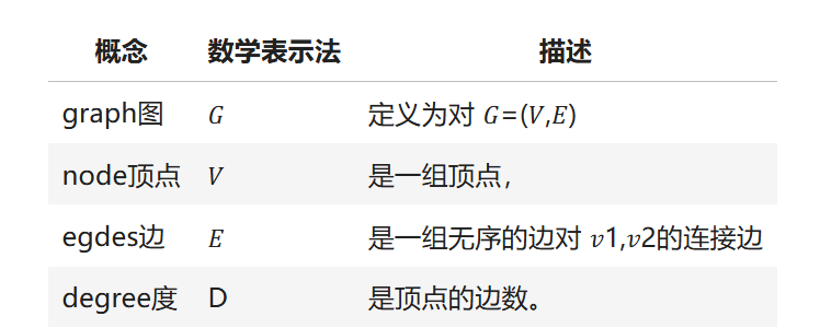
在下面的笔记流程中,将始终使|用 Graph 𝐺,节点集 𝑉 和边集 𝐸。
节点简单来说就是样本,边就是样本和样本之间的关系。
⚙️ 全局设置
为了防止 运行的效果不固定等随机性的问题,要固定一下随机数,种子等参数。
RANDOM_STATE = 42
NUM_EPOCHS = 100
自定义函数
def set_seed_for_torch(seed):
    torch.manual_seed(seed)
    if torch.cuda.is_available():
        torch.cuda.manual_seed(seed)      # For single-GPU.
        torch.cuda.manual_seed_all(seed)  # For multi-GPU.
    torch.backends.cudnn.deterministic = True
    torch.backends.cudnn.benchmark = False

def set_seed_for_numpy(seed):
    np.random.seed(seed)

def set_seed_for_random(seed):
    random.seed(seed)
设置使用
set_seed_for_torch(RANDOM_STATE)
set_seed_for_numpy(RANDOM_STATE)
set_seed_for_random(RANDOM_STATE)
📜 数据概述
先来了解一下数据
elliptic_txs_features = pd.read_csv('elliptic_txs_features.csv', header=None)
elliptic_txs_classes = pd.read_csv('elliptic_txs_classes.csv')
elliptic_txs_edgelist = pd.read_csv('elliptic_txs_edgelist.csv')
elliptic_txs_features.columns = ['txId'] + [f'V{i}' for i in range(1, 167)]
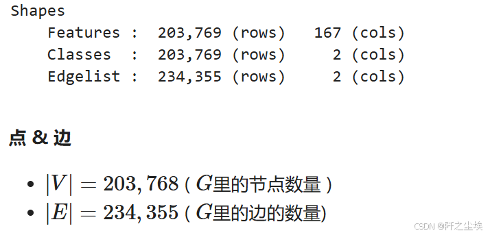
print(f"""Shapes
{4*' '}Features : {elliptic_txs_features.shape[0]:8,} (rows) {elliptic_txs_features.shape[1]:4,} (cols)
{4*' '}Classes : {elliptic_txs_classes.shape[0]:8,} (rows) {elliptic_txs_classes.shape[1]:4,} (cols)
{4*' '}Edgelist : {elliptic_txs_edgelist.shape[0]:8,} (rows) {elliptic_txs_edgelist.shape[1]:4,} (cols)
""")
特征矩阵
elliptic_txs_features.head(3) # 节点特征x,也就是每一笔交易的特征变量,这里脱敏了,用V1-V167代表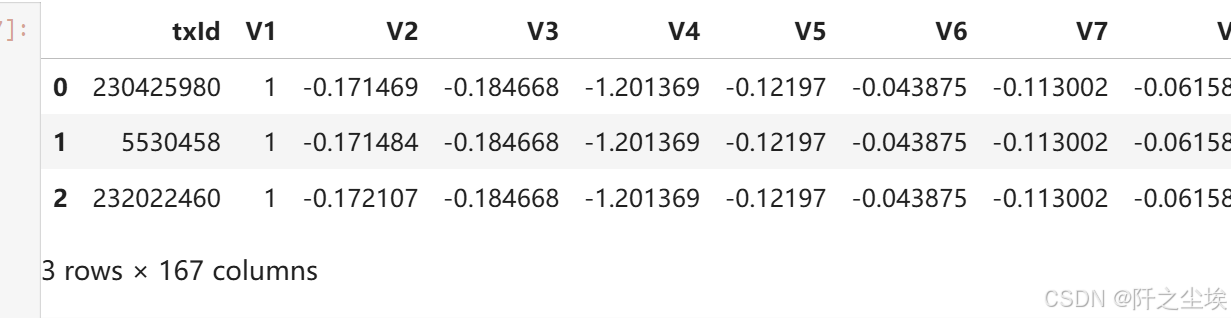
响应变量
elliptic_txs_classes.head(3) # 节点的类别y,其实可以和上面合并的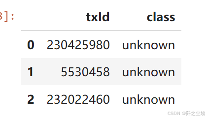
其实普通的表格数据就是上面这些,X和y就可以了,但是图数据就是会有连接,就是下面的边
边的关系
elliptic_txs_edgelist.head(3) # 边的关系,表示这两笔交易有关系,这也是图数据特有的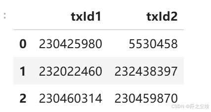
所以可以看到 图数据跟平常使用的二维数据最大的差别就在于它有边的数据关系。这个边的数据关系就是一个形状为(n,2)的矩阵。其他的特征矩阵x跟响应变量y都是一样的。
一般来说边关系也就是顶点顶点之间的关系。放在这个数据上的例子就是每一笔交易跟另外一笔交易之间是有联系的,怎么构建这个联系?有可能是他们拥有相同的交易账户,也有可能是使用了相同的交易渠道等等(这就涉及到图数据中的建边的方法了,非常多。有同构异构,硬介质,弱介质),这个边的关系是可以自己想方法构建的,但是这个数据集自带的边的关系,我们也不知道他怎么构建的,用就行了。
查看一下类别分布class.
elliptic_txs_classes['class_mapped'] = elliptic_txs_classes['class'].replace({'1': 'illicit', '2': 'licit'})

percentage_distribution = round(100 * elliptic_txs_classes['class_mapped'].value_counts(normalize=True), 2)
class_counts = elliptic_txs_classes['class_mapped'].value_counts()

emoji_mapping = {'licit': '✅', 'illicit': '❌', 'unknown': '🤷'}
elliptic_txs_classes['emoji'] = elliptic_txs_classes['class_mapped'].map(emoji_mapping)

classes_df = pd.DataFrame({
    'Class Mapped': elliptic_txs_classes['class_mapped'].unique(),
    'Class Raw': elliptic_txs_classes['class'].unique(),
    'Counts': class_counts.to_numpy(),
    'Percentage': percentage_distribution.to_numpy(),
    'Emoji': [emoji_mapping[class_label] for class_label in elliptic_txs_classes['class_mapped'].unique()]
})
classes_df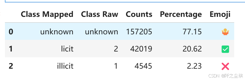
-
77.15% 的类别是 unknown 未定义
-
20.62% 的类别是 licit (2) 合法
-
2.23% 的类别是 illicit (1) 不合法
num_nodes = elliptic_txs_features.shape[0]
num_edges = elliptic_txs_edgelist.shape[0]

print(f"nodes节点数量: {num_nodes:,}")
print(f"edges边的数量: {num_edges:,}")
简单分析
# 使用nx构图
G = nx.from_pandas_edgelist(elliptic_txs_edgelist, 'txId1', 'txId2')
🔍(EDA) 探索性分析
## 图整体的情况,边和节点数量
plt.figure(figsize=(4, 4),dpi=108)
sizes = [num_nodes, num_edges]
labels = ['Nodes', 'Edges']
colors = ['skyblue', 'salmon']
plt.pie(sizes, labels=labels, colors=colors, autopct='%1.1f%%', startangle=140,
        wedgeprops = {'edgecolor' : 'black',
                      'linewidth': 2,
                      'antialiased': True})
plt.title('Basic Graph Properties')
plt.axis('equal')
plt.show()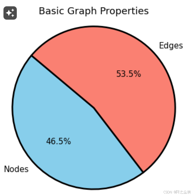
# ---度的分布,由于肯定是一个右偏分布,所以用对数轴---
plt.figure(figsize=(6, 4),dpi=128)
degrees = [G.degree(n) for n in G.nodes()]
plt.hist(degrees, bins=50, log=True, color='skyblue', edgecolor='black', linewidth=2.0)
plt.xscale('log')
plt.yscale('log')
plt.title('Degree Distribution (Log-Log Scale)')
plt.xlabel('Degree (log)')
plt.ylabel('Number of Nodes (log)')
plt.show()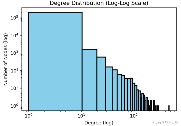
大部分的度都在0和1附近,也就是孤立的节点,少数有100个及以上的节点,这肯定就是团伙了。
📊 基础统计
# 简单采样分析
classes_sampled = elliptic_txs_classes.groupby('class_mapped').sample(frac=0.05, random_state=RANDOM_STATE)
txIds_sampled = classes_sampled['txId']

# 根据采样的 txIds 过滤 elliptic_txs_edgelist
edgelist_sampled = elliptic_txs_edgelist[
    elliptic_txs_edgelist['txId1'].isin(txIds_sampled) | elliptic_txs_edgelist['txId2'].isin(txIds_sampled)
]

# 根据采样的 txIds 过滤 elliptic_txs_features
features_sampled = elliptic_txs_features[elliptic_txs_features['txId'].isin(txIds_sampled)]

print(f"Sampled Classes:\n{classes_sampled['class_mapped'].value_counts()}\n")
print(f"Sampled Edgelist: {edgelist_sampled.shape[0]:,}")
print(f"Sampled Features: {features_sampled.shape[0]:,}")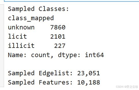
原始数据20w,太大了,我们取了5%的数据,大概1w条,最后样本里面的合法交易的2.1k,未定义的7.8k,不合法的是227条。
# 边和节点数
num_nodes = features_sampled.shape[0]
num_edges = edgelist_sampled.shape[0]

print(f"Number of nodes: {num_nodes:,}")
print(f"Number of edges: {num_edges:,}")

# 度的分布
plt.figure(figsize=(7, 4),dpi=128)

node_degrees = edgelist_sampled['txId1'].value_counts() + edgelist_sampled['txId2'].value_counts()
node_degrees.hist(bins=50, edgecolor='black')
plt.title('Distribution of Node Degrees')
plt.xlabel('Degree')
plt.ylabel('Number of Nodes')
plt.grid(False)
plt.show()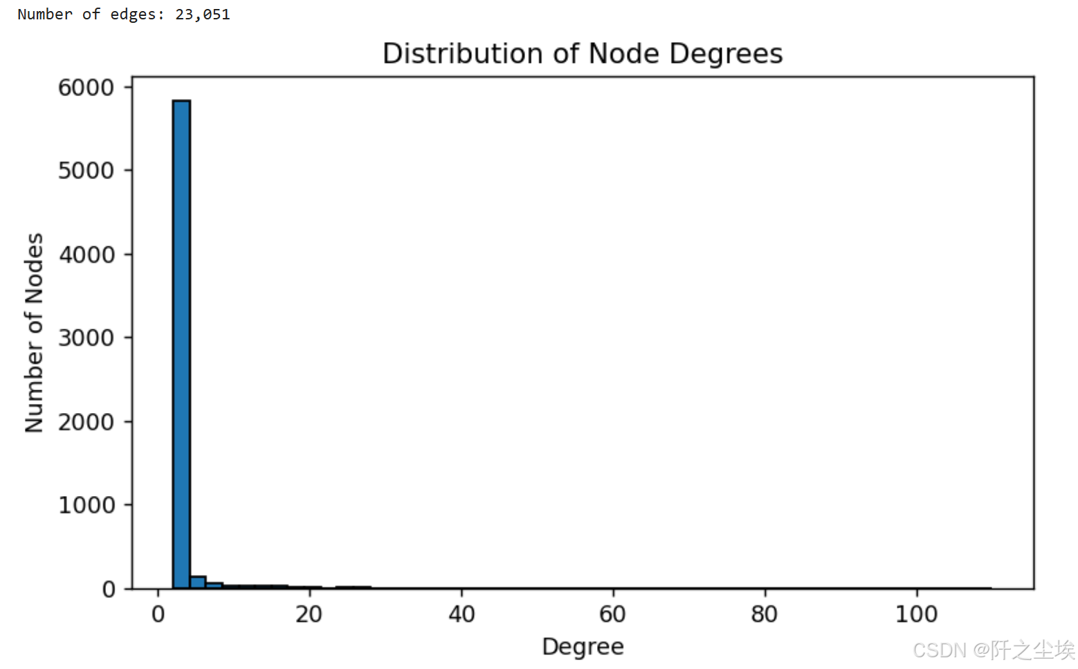
不用对数轴就是一个及其严重的右偏分布
🔗图连接
# 构图
G = nx.from_pandas_edgelist(edgelist_sampled, 'txId1', 'txId2')
# --- 连接组件,极大连通子图 ---
num_connected_components = nx.number_connected_components(G)
print(f"Number of connected components: {num_connected_components}")

# --- 最大的连接,最大的极大连通子图  ---
giant_component = max(nx.connected_components(G), key=len)
G_giant = G.subgraph(giant_component)

print(f"Giant component - Number of nodes: {G_giant.number_of_nodes():,}")
print(f"Giant component - Number of edges: {G_giant.number_of_edges():,}")
number_connected_components这个函数计算图 G 中的连接组件的数量。 连接组件是图中所有节点之间都有路径相连的最大子图。换句话说,一个连接组件包含能够彼此到达的所有节点,即:极大连通子图。
max(nx.connected_components(G), key=len):通过 max 和 key=len 找到包含节点最多的连接组件,即最大的极大连通子图,也就是找最大的团伙. 这个最大的团伙有400个节点,431条边。
# 最大团伙里面的最短路径长度分布 #
path_lengths = dict(nx.shortest_path_length(G_giant))
path_lengths_values = [length for target_lengths in path_lengths.values() for length in target_lengths.values()]

plt.figure(figsize=(7, 4),dpi=128)
plt.hist(path_lengths_values, bins=50, edgecolor='black')
plt.title('Shortest Path Length Distribution in Giant Component')
plt.xlabel('Path Length')
plt.ylabel('Frequency')
plt.show()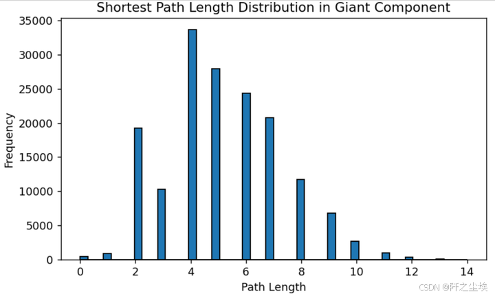
一个节点需要通过几条边才能找到另外一个节点,就是路径长度,上面的图是这个最大的团伙里面的最小路径长度的分布, 可以看到基本上再4和5附近,也就是说一个交易一般通过最多4-5个交易就能关联上,
🎯节点中心性度量
在本节中,我们将研究节点中心性度量。这些度量在图论中用于识别网络中最重要或最有影响力的节点。我们将重点关注以下三个中心性指标:
🔢 度中心性(Degree centrality)
定义: 度中心性衡量节点在网络中拥有的直接连接数。它被定义为连接到节点的边数。

解释: 具有高度中心性的节点是高度连接的,并且通过与许多其他节点直接交互,可能在网络中发挥关键作用。 简而言之,团伙头目,团伙里面认识最多的人。
🔀 中介中心性(Betweenness centrality.)
定义: 中介中心性衡量节点位于网络中其他节点之间的最短路径上的程度。
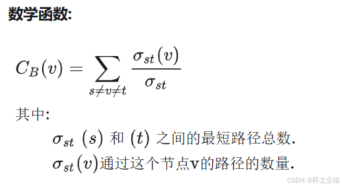
其中和之间的最短路径总数通过这个节点的路径的数量CB(v)=∑s≠v≠tσst(v)σst其中:σst(s)和(t)之间的最短路径总数.σst(v)通过这个节点v的路径的数量.
解释: 具有高中介中心性的节点对网络中的信息或资源流具有重要控制权,因为它连接网络的不同部分。它通常表示对通信至关重要的节点。 简而言之,团伙联系人,团伙里面的人和组织都是通过他来进行联系控制的。
🌐 接近中心性(Closeness centrality)
定义: 接近中心性衡量一个节点与网络中所有其他节点的距离。它是从节点到网络中所有其他节点的最短路径距离之和的倒数。
数学函数:
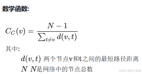
解释: 具有高接近中心性的节点可以与所有其他节点快速交互,并且可以成为信息或影响整个网络的有效传播者。 简而言之,团伙情报员,团伙里面的人都是通过他来进行最短的联系的。
下面一一计算:
# Degree centrality.度中心性
degree_centrality = nx.degree_centrality(G_giant)
top_degree_centrality = sorted(degree_centrality.items(), key=lambda x: x[1], reverse=True)[:10]
df_top_degree_centrality = pd.DataFrame(top_degree_centrality, columns=['Node', 'Degree Centrality'])

print("Top 10 nodes by degree centrality:")
print("==================================")
print(df_top_degree_centrality)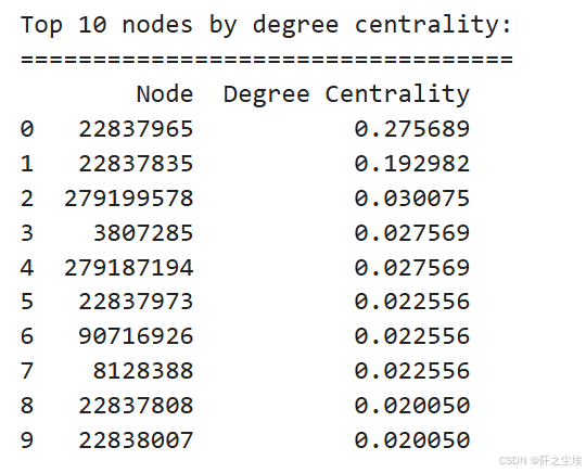
22837965 ,22837835,这两个交易关联了特别多别的交易
top_nodes_by_ = df_top_degree_centrality['Node'].tolist()
subgraph = G_giant.subgraph(top_nodes_by_)
node_color = [degree_centrality[node] for node in subgraph.nodes()]
norm = mpl.colors.Normalize(vmin=min(node_color), vmax=max(node_color))
node_color_normalized = [norm(value) for value in node_color]
cmap = plt.cm.cool

# -------- #
# Plotting #
# -------- #
plt.figure(figsize=(7, 3),dpi=128)
nx.draw(subgraph, with_labels=True, node_size=500, edge_color='gray', font_size=8,
        node_color=node_color_normalized, cmap=cmap)
plt.title('Top 10 Degree Centrality Nodes')
plt.colorbar(mpl.cm.ScalarMappable(norm=norm, cmap=cmap), label='Degree Centrality')
plt.show()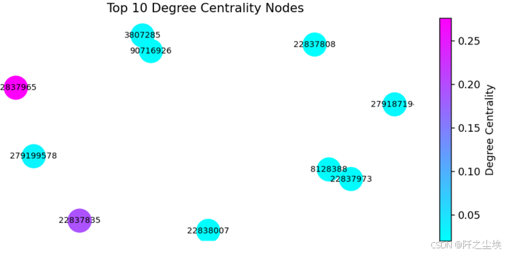
# Betweenness centrality. 中介中心性
betweenness_centrality = nx.betweenness_centrality(G_giant)
top_betweenness_centrality = sorted(betweenness_centrality.items(), key=lambda x: x[1], reverse=True)[:10]
df_top_betweenness_centrality = pd.DataFrame(top_betweenness_centrality, columns=['Node', 'Betweenness Centrality'])

print("Top 10 nodes by betweenness centrality:")
print("=======================================")
print(df_top_betweenness_centrality)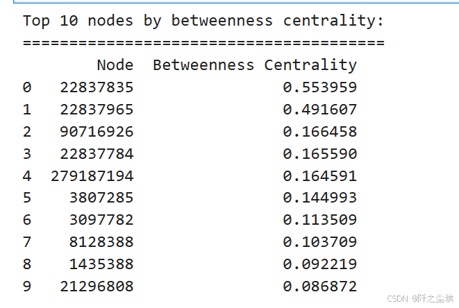
# Plotting #

top_nodes_by_ = df_top_betweenness_centrality['Node'].tolist()
subgraph = G_giant.subgraph(top_nodes_by_)
node_color = [betweenness_centrality[node] for node in subgraph.nodes()]
norm = mpl.colors.Normalize(vmin=min(node_color), vmax=max(node_color))
node_color_normalized = [norm(value) for value in node_color]
cmap = plt.cm.cool

plt.figure(figsize=(7, 3),dpi=128)

nx.draw(subgraph, with_labels=True, node_size=300, edge_color='gray', font_size=8,
        node_color=node_color_normalized, cmap=cmap)
plt.title('Top 10 Betweenness Centrality Nodes')
plt.colorbar(mpl.cm.ScalarMappable(norm=norm, cmap=cmap), label='Betweenness Centrality')
plt.show()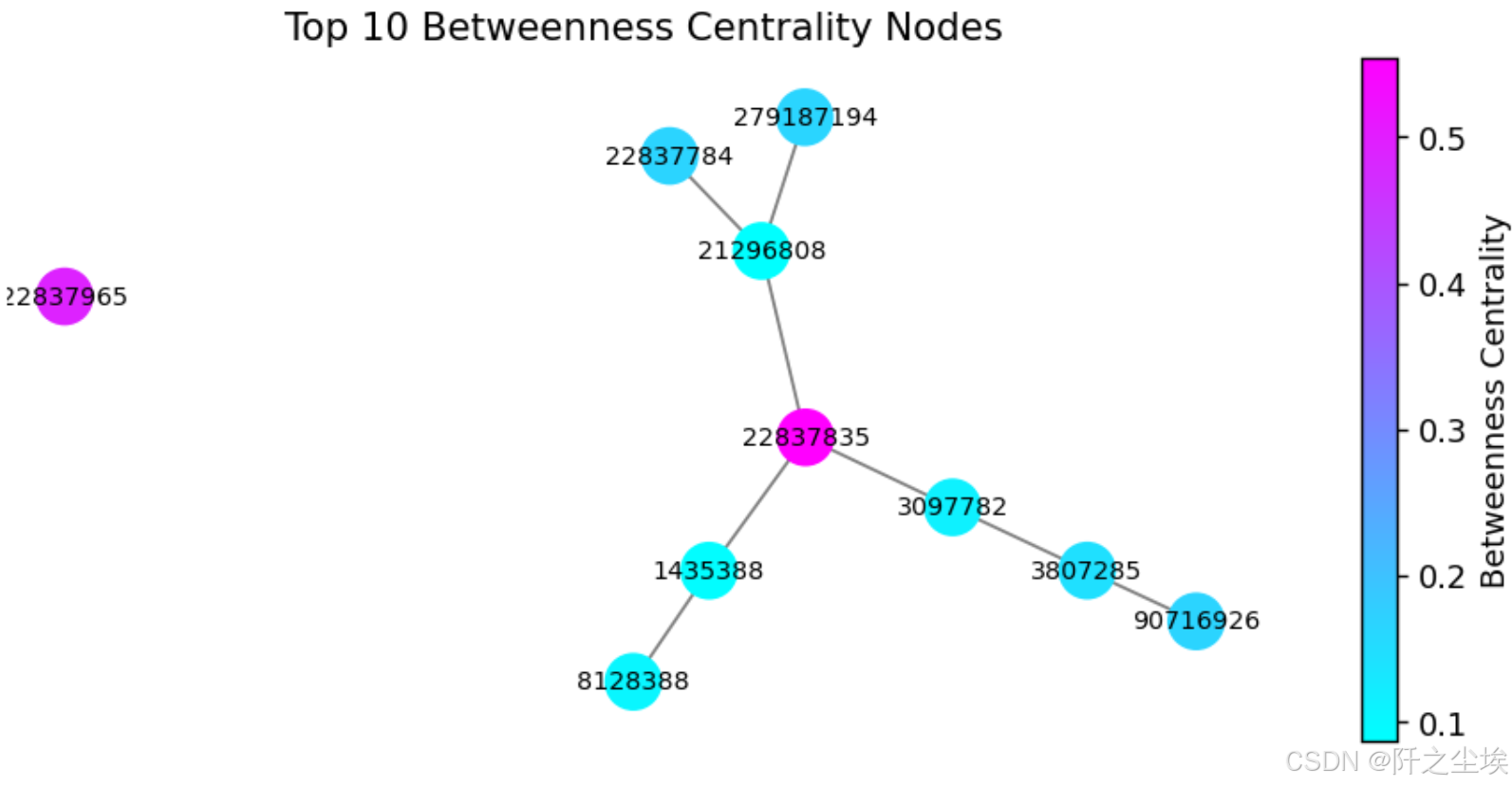
# Closeness centrality. 接近中心性
closeness_centrality = nx.closeness_centrality(G_giant)
top_closeness_centrality = sorted(closeness_centrality.items(), key=lambda x: x[1], reverse=True)[:10]
df_top_closeness_centrality = pd.DataFrame(top_closeness_centrality, columns=['Node', 'Closeness Centrality'])

print("Top 10 nodes by closeness centrality:")
print("=====================================")
print(df_top_closeness_centrality)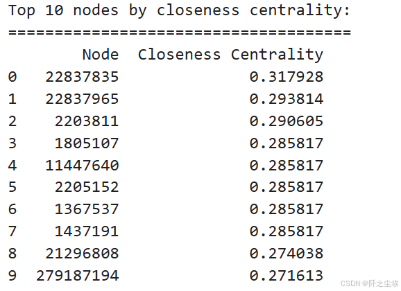
top_nodes_by_closeness = df_top_closeness_centrality['Node'].tolist()
subgraph = G_giant.subgraph(top_nodes_by_closeness)
node_color = [closeness_centrality[node] for node in subgraph.nodes()]
norm = mpl.colors.Normalize(vmin=min(node_color), vmax=max(node_color))
node_color_normalized = [norm(value) for value in node_color]
cmap = plt.cm.cool

# Plotting #
# -------- #
plt.figure(figsize=(7, 3),dpi=128)

nx.draw(subgraph, with_labels=True, node_size=300, edge_color='gray', font_size=8,
        node_color=node_color_normalized, cmap=cmap)
plt.title('Top 10 Closeness Centrality Nodes')
plt.colorbar(mpl.cm.ScalarMappable(norm=norm, cmap=cmap), label='Closeness Centrality')
plt.show()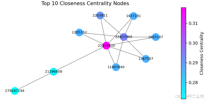
🖼️ 图的可视化
对采样出来的图进行可视化
# --------- #
# Preparing #

# 识别在每种中心度量中排名靠前的节点及其组合
top_nodes_degree = set([node for node, _ in top_degree_centrality])
top_nodes_betweenness = set([node for node, _ in top_betweenness_centrality])
top_nodes_closeness = set([node for node, _ in top_closeness_centrality])

top_nodes_both = top_nodes_degree.intersection(top_nodes_betweenness)
top_nodes_closeness_and_degree = top_nodes_closeness.intersection(top_nodes_degree)
top_nodes_closeness_and_betweenness = top_nodes_closeness.intersection(top_nodes_betweenness)
top_nodes_all_three = top_nodes_closeness.intersection(top_nodes_degree).intersection(top_nodes_betweenness)

# 根据中心度量分配颜色和形状。
node_color = []  ;  node_shape = []

for node in G_giant.nodes():
    if node in top_nodes_all_three:
        node_color.append('purple')
        node_shape.append('D')
    elif node in top_nodes_closeness_and_degree:
        node_color.append('orange')
        node_shape.append('h')
    elif node in top_nodes_closeness_and_betweenness:
        node_color.append('cyan')
        node_shape.append('v')
    elif node in top_nodes_both:
        node_color.append('green')
        node_shape.append('s')
    elif node in top_nodes_degree:
        node_color.append('red')
        node_shape.append('o')
    elif node in top_nodes_betweenness:
        node_color.append('magenta')
        node_shape.append('^')
    elif node in top_nodes_closeness:
        node_color.append('yellow')
        node_shape.append('h')
    else:
        node_color.append('slategrey')
        node_shape.append('o')

# -------- #
# Plotting #
# -------- #

plt.figure(figsize=(15, 11))

pos = nx.spring_layout(G_giant)
# Draw all nodes first.
nx.draw_networkx_nodes(G_giant, pos, node_color='slategrey', node_size=10)

# Draw nodes with specific centrality measures.
nx.draw_networkx_nodes(G_giant, pos, nodelist=list(top_nodes_degree - top_nodes_both - top_nodes_closeness_and_degree),
                       node_color='red', node_size=50, node_shape='o',
                       label='Degree Centrality')
nx.draw_networkx_nodes(G_giant, pos, nodelist=list(top_nodes_betweenness - top_nodes_both - top_nodes_closeness_and_betweenness),
                       node_color='magenta', node_size=50, node_shape='^',
                       label='Betweenness Centrality')
nx.draw_networkx_nodes(G_giant, pos, nodelist=list(top_nodes_closeness - top_nodes_closeness_and_degree - top_nodes_closeness_and_betweenness),
                       node_color='gold', node_size=50, node_shape='h',
                       label='Closeness Centrality')
nx.draw_networkx_nodes(G_giant, pos, nodelist=list(top_nodes_both),
                       node_color='green', node_size=80, node_shape='s',
                       label='Degree & Betweenness Centrality')
nx.draw_networkx_nodes(G_giant, pos, nodelist=list(top_nodes_closeness_and_degree),
                       node_color='orange', node_size=70, node_shape='h',
                       label='Degree & Closeness Centrality')
nx.draw_networkx_nodes(G_giant, pos, nodelist=list(top_nodes_closeness_and_betweenness),
                       node_color='cyan', node_size=70, node_shape='v',
                       label='Betweenness & Closeness Centrality')
nx.draw_networkx_nodes(G_giant, pos, nodelist=list(top_nodes_all_three),
                       node_color='purple', node_size=100, node_shape='D',
                       label='Closeness, Degree, & Betweenness Centrality')

# Draw edges.
nx.draw_networkx_edges(G_giant, pos, width=0.8, edge_color='gray', alpha=0.5)

plt.axis('off')
plt.title('Nodes Highlighted by Degree, Betweenness, and Closeness Centrality')
plt.legend(scatterpoints=1)
plt.show()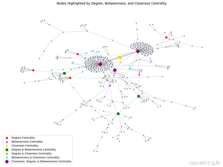
红色圆圈(Degree Centrality):这些节点通过度中心性度量表现出色,表示这些节点有最多的直接连接。换句话说,这些节点在网络中是高度连接的,可能代表了交易频率较高的账户或实体。
紫红色三角形(Betweenness Centrality):这些节点通过中介中心性表现出色,表明它们在网络中的桥梁作用较大,即通过它们的路径很多。这可能意味着这些节点在不同部分的交易之间起到了重要的中介作用。
黄色六边形(Closeness Centrality):这些节点通过接近中心性度量表现出色,意味着它们可以通过最少的跳数或交易步骤触及网络的其他节点。可能意味着这些节点在整个网络中的传播效率更高。
绿色方块(Degree & Betweenness Centrality):这些节点既在度中心性上得分高,也在中介中心性上得分高,表明它们不仅与其他节点有很多连接,而且在不同部分之间起到了桥梁的作用。
橙色六边形(Degree & Closeness Centrality):这些节点既在度中心性上得分高,也在接近中心性上得分高,表明它们在网络中的位置不仅与很多节点连接,还可以通过较短的路径触及网络中的大部分其他节点。
青色倒三角形(Betweenness & Closeness Centrality):这些节点既在中介中心性上得分高,也在接近中心性上得分高,说明它们在桥梁作用和全局接触效率上都表现突出。
紫色菱形(Closeness, Degree, & Betweenness Centrality):这些节点在三种度量上都得分高,是网络中最重要的节点,既连接广泛,又起桥梁作用,还能有效触及网络的其他部分。这些节点可能是最关键的交易节点,影响网络的整体结构。
从网络布局来看,图中似乎存在一些明显的集群或子结构,表明交易网络中存在几种紧密相关的交易群体。而上述这些高中心性节点可能在这些群体之间或群体内部起到了重要的作用。
📈 具体类别分析
# 子图类别
illicit_nodes = classes_sampled[classes_sampled['class_mapped'] == 'illicit']['txId']
licit_nodes = classes_sampled[classes_sampled['class_mapped'] == 'licit']['txId']

G_illicit = G.subgraph(illicit_nodes)
G_licit = G.subgraph(licit_nodes)
classes_df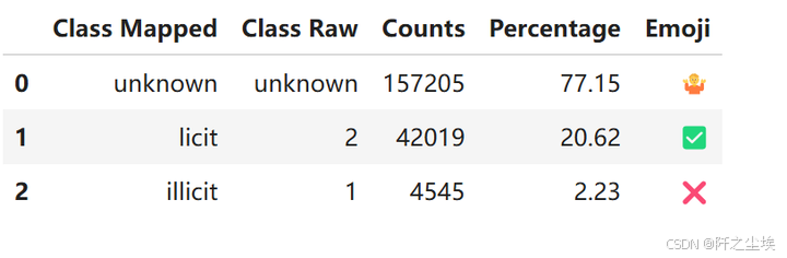
分开可视化
plt.figure(figsize=(12, 6),dpi=108)

plt.subplot(1, 2, 1)
nx.draw(G_illicit, with_labels=False, node_size=10, node_color='indianred', edge_color='black')
plt.title('Illicit Transactions Subgraph')

plt.subplot(1, 2, 2)
nx.draw(G_licit, with_labels=False, node_size=10, node_color='forestgreen', edge_color='black')
plt.title('Licit Transactions Subgraph')

plt.show()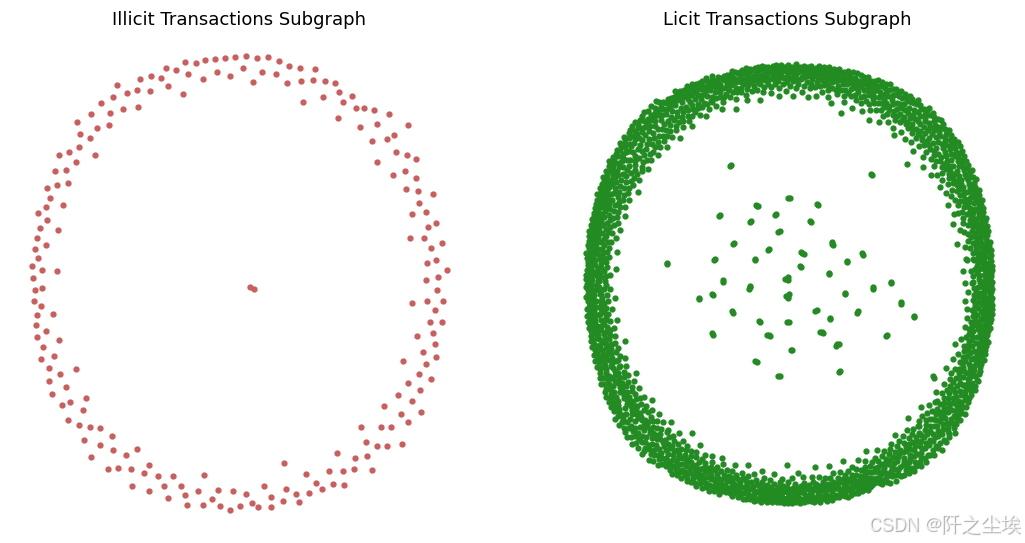
❌ 不合法交易的 图
-
节点分布相当稀疏,呈环状分布。
-
大多数节点位于外围,少数节点集中在中心。
-
这表明__非法交易的相互联系可能较少__,少数中心节点可能充当网络的枢纽_或关键点。
✅ 合法交易的图
-
节点密度越高,表明网络越复杂,实体间的交易或互动越多。
-
可能意味着网络更成熟或更合法。
-
表明合法交易可能涉及更多相互关联的实体,许多节点关系密切或互动更频繁。
👥 社区检测
社群检测的目的是在图中识别节点内部连接比与图的其他部分连接更密集的集群或社群。
#计算最佳分区 ( 基于鲁文算法)
partition = community_louvain.best_partition(G_giant)

# 画图
plt.figure(figsize=(10, 8),dpi=128)

pos = nx.spring_layout(G_giant)
cmap = plt.get_cmap('viridis')
nx.draw_networkx_nodes(G_giant, pos, node_color=list(partition.values()), node_size=8, cmap=cmap)
nx.draw_networkx_edges(G_giant, pos, alpha=0.5, edge_color='grey')
plt.axis('off')

plt.show()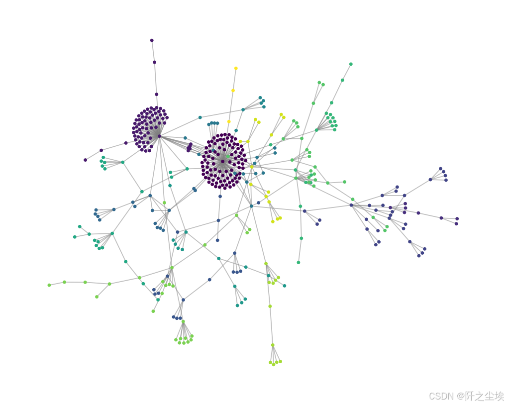
不同颜色属于一类,可以看到紫色类的团伙明显密集一些。
社区划分:每个节点的颜色代表了它所属的社区,颜色不同的节点表示它们属于不同的社区。可以看出,图中的节点被分成了若干个社区,每个社区在图中呈现为一组高度连接的节点。Louvain 算法将这些节点分组,从而揭示出网络中的局部结构。
节点集中度:图中有两个较大的紫色社区,它们在图的左下方和右侧非常集中。这表明这两个社区内部的节点彼此之间有较多的连接,是网络中的核心部分,可能代表一些交易密集的群体或子结构。
连接分布:图中的其他社区以不同颜色分布在网络的各个区域,可以看到这些节点之间的连接相对较少,或是这些社区之间的连接较为稀疏。这种结构表明,不同的社区之间存在一定的隔离,某些社区可能更集中于特定的交易活动。
🧠 图神经网络
图神经网络(GNN)是一种专为图数据设计的深度学习技术,适用于节点分类、图分类或边的预测等任务。在我们的例子中,目前我们将执行____节点预测____。
device = torch.device('cuda' if torch.cuda.is_available() else 'cpu')
device
### 三种图神经网络,准备3套评价指标
metrics_per_gnn = {
    'gcn': {
        'val': {
            'precisions': [],
            'probas': [],
        },
        'test': {
            'licit': {
                'probas': []
            },
            'illicit': {
                'probas': []
            },
        }
    },
    'gat': {
        'val': {
            'precisions': [],
            'probas': [],
        },
        'test': {
            'licit': {
                'probas': []
            },
            'illicit': {
                'probas': []
            },
        }
    },
    'gin': {
        'val': {
            'precisions': [],
            'probas': [],
        },
        'test': {
            'licit': {
                'probas': []
            },
            'illicit': {
                'probas': []
            },
        }
    }
}
🛠️ 准备工作
查看数据量
num_edges = elliptic_txs_edgelist.shape[0]
num_nodes = elliptic_txs_features.shape[0]

print(f'Number of edges in the graph: {num_edges:8,}')
print(f'Number of nodes in the graph: {num_nodes:8,}')
# 创建以 txId 为键、实际索引为值的映射 #
tx_id_mapping = {tx_id: idx for idx, tx_id in enumerate(elliptic_txs_features['txId'])}

edges_with_features = elliptic_txs_edgelist[elliptic_txs_edgelist['txId1'].isin(list(tx_id_mapping.keys()))\
                                          & elliptic_txs_edgelist['txId2'].isin(list(tx_id_mapping.keys()))]

edges_with_features['Id1'] = edges_with_features['txId1'].map(tx_id_mapping)
edges_with_features['Id2'] = edges_with_features['txId2'].map(tx_id_mapping)

edges_with_features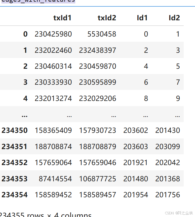
边的索引
edge_index = torch.tensor(edges_with_features[['Id1', 'Id2']].values.T, dtype=torch.long)
edge_index
# 以合适的格式保存节点特征

node_features = torch.tensor(elliptic_txs_features.drop(columns=['txId']).values,
                             dtype=torch.float)
print(node_features.shape)
node_features[:2]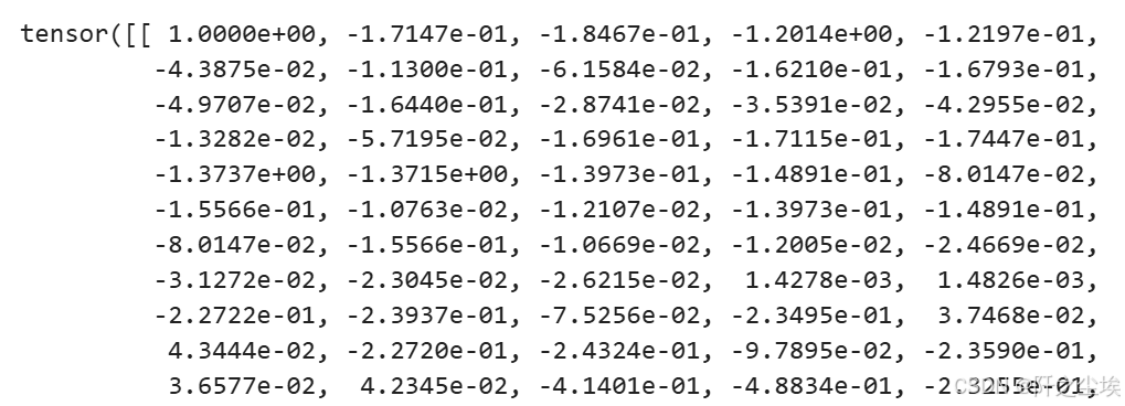
-
第一个维度描述了# nodes
-
第二个维度描述了 # node features
elliptic_txs_classes['class'].value_counts()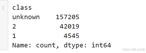
# 类别标签编码  Labelencode target class #

le = LabelEncoder()
class_labels = le.fit_transform(elliptic_txs_classes['class'])
node_labels = torch.tensor(class_labels, dtype=torch.long)
original_labels = le.inverse_transform(class_labels)

print(original_labels)
print(class_labels)
print(node_labels)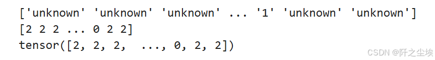
print(le.inverse_transform([0])) # illicit
print(le.inverse_transform([1])) # licit
print(le.inverse_transform([2])) # unknown
# 放入 pytorch geometric 的数据对象里面 #
data = Data(x=node_features,
            edge_index=edge_index,
            y=node_labels)

# Move data to GPU.
data = data.to(device)
现在创建了geometric 的数据结构 pytorch geometric Data object.
但是,在这个对象中,我们仍然有很多_未知_ 🤷 ,我们不想在这些节点上训练我们的 GNN。我们只想在已知节点上进行训练,即那些_licit_ ✅ 或 illicit ❌ 的节点。
把位未知的标签的数据进行掩码
## 未知的数据掩码掉
known_mask = (data.y == 0) | (data.y == 1) # 只要已知的标签 licit or illicit
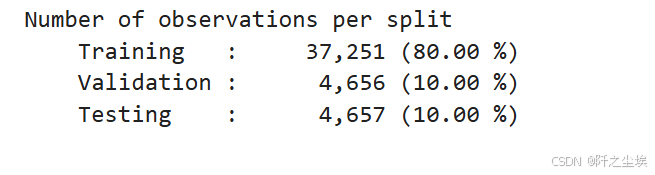
unknown_mask = data.y == 2 # 未知标签掩码划分训练集,验证集,测试集
#定义训练集,验证集,测试集

num_known_nodes = known_mask.sum().item()
permutations = torch.randperm(num_known_nodes)
train_size = int(0.8 * num_known_nodes)      #8成训练
val_size = int(0.1 * num_known_nodes)        #1成验证
test_size = num_known_nodes - train_size - val_size  #1验测试
total = np.sum([train_size, val_size, test_size])

print(f"""Number of observations per split
    Training   : {train_size:10,} ({100*train_size/total:0.2f} %)
    Validation : {val_size:10,} ({100*val_size/total:0.2f} %)
    Testing    : {test_size:10,} ({100*test_size/total:0.2f} %)
""")
#为 Train、Val、Test 的索引创建掩码

data.train_mask = torch.zeros(data.num_nodes, dtype=torch.bool)
data.val_mask = torch.zeros(data.num_nodes, dtype=torch.bool)
data.test_mask = torch.zeros(data.num_nodes, dtype=torch.bool)

train_indices = known_mask.nonzero(as_tuple=True)[0][permutations[:train_size]]
val_indices = known_mask.nonzero(as_tuple=True)[0][permutations[train_size:train_size + val_size]]
test_indices = known_mask.nonzero(as_tuple=True)[0][permutations[train_size + val_size:]]

data.train_mask[train_indices] = True
data.val_mask[val_indices] = True
data.test_mask[test_indices] = True

data.train_mask
查看删除后,用于训练的数据情况
# 数据集统计 #

train_licit, train_illicit = (data.y[data.train_mask] == 1).sum().item(), (data.y[data.train_mask] == 0).sum().item()
val_licit, val_illicit = (data.y[data.val_mask] == 1).sum().item(), (data.y[data.val_mask] == 0).sum().item()
test_licit, test_illicit = (data.y[data.test_mask] == 1).sum().item(), (data.y[data.test_mask] == 0).sum().item()

# C计算总量
train_total = train_licit + train_illicit
val_total = val_licit + val_illicit
test_total = test_licit + test_illicit

# 百分比
train_licit_pct = (train_licit / train_total) * 100
train_illicit_pct = (train_illicit / train_total) * 100
val_licit_pct = (val_licit / val_total) * 100
val_illicit_pct = (val_illicit / val_total) * 100
test_licit_pct = (test_licit / test_total) * 100
test_illicit_pct = (test_illicit / test_total) * 100

pd.DataFrame({
    'Set': ['Training', 'Validation', 'Testing'],
    'Total Count': [train_total, val_total, test_total],
    'Licit': [train_licit, val_licit, test_licit],
    'Licit (%)': [train_licit_pct, val_licit_pct, test_licit_pct],
    'Illicit': [train_illicit, val_illicit, test_illicit],
    'Illicit (%)': [train_illicit_pct, val_illicit_pct, test_illicit_pct]
})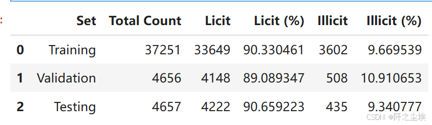
每个数据集里面的黑白占比类似,PSI稳定,正好
mapped_classes = np.array(['illicit', 'licit'])🛠️ 组件函数
在进行神经网络的训练评估之前,我们首先要定义一些通用的函数,方便复用。
评估用的
# Training, Evaluation and prediction methods #

def compute_metrics(y_true, y_pred):
    """计算并返回精度、召回率和F1分数"""
    precision = precision_score(y_true, y_pred, average='weighted', zero_division=0)
    recall = recall_score(y_true, y_pred, average='weighted', zero_division=0)
    f1 = f1_score(y_true, y_pred, average='weighted', zero_division=0)
    return precision, recall, f1

def train(model, data, optimizer, criterion):
    model.train()
    optimizer.zero_grad()
    out = model(data)
    loss = criterion(out[data.train_mask], data.y[data.train_mask])
    loss.backward()
    optimizer.step()
    return loss.item()

def evaluate(model, data, mask):
    model.eval()
    with torch.no_grad():
        out = model(data)
        pred = out.argmax(dim=1)

        correct = (pred[mask] == data.y[mask]).sum().item()
        accuracy = correct / mask.sum().item()

        y_true = data.y[mask].cpu().numpy()     ;     y_pred = pred[mask].cpu().numpy()

        precision, recall ,  f1 = train_prec, train_rec, train_f1 = compute_metrics(y_true_train, y_pred_train)
        metrics = { 'accuracie': accuracy,'precision': precision,  'recall': recall,  'f1_score': f1   }

    return metrics

def predict(model, data):
    model.eval()
    with torch.no_grad():
        out = model(data)
        pred = out.argmax(dim=1)
    return pred

def predict_probabilities(model, data):
    model.eval()
    with torch.no_grad():
        out = model(data)
        probabilities = torch.exp(out)
    return probabilities
训练图神经网络用的:
from sklearn.metrics import precision_score, recall_score, f1_score

def train_gnn(num_epochs, data, model, optimizer, criterion):

    metrics = {
        'train': {'losses': [], 'accuracies': [], 'precisions': [], 'recalls': [], 'f1_scores': []},
        'val': {'accuracies': [], 'precisions': [], 'recalls': [], 'f1_scores': []}
    }

    for epoch in range(1, num_epochs + 1):
        model.train()
        optimizer.zero_grad()
        out = model(data)
        loss = criterion(out[data.train_mask], data.y[data.train_mask])
        loss.backward()
        optimizer.step()

        # --- Calculate training metrics ---
        pred_train = out[data.train_mask].argmax(dim=1)
        correct_train = (pred_train == data.y[data.train_mask]).sum()
        train_acc = int(correct_train) / int(data.train_mask.sum())

        y_true_train = data.y[data.train_mask].cpu().numpy()
        y_pred_train = pred_train.cpu().numpy()
        train_prec, train_rec, train_f1 = compute_metrics(y_true_train, y_pred_train)

        metrics['train']['losses'].append(loss.item())
        metrics['train']['accuracies'].append(train_acc)
        metrics['train']['precisions'].append(train_prec)
        metrics['train']['recalls'].append(train_rec)
        metrics['train']['f1_scores'].append(train_f1)

        # --- Validate and calculate validation metrics ---
        model.eval()
        with torch.no_grad():
            out = model(data)
            pred_val = out[data.val_mask].argmax(dim=1)
            correct_val = (pred_val == data.y[data.val_mask]).sum()
            val_acc = int(correct_val) / int(data.val_mask.sum())

            y_true_val = data.y[data.val_mask].cpu().numpy()
            y_pred_val = pred_val.cpu().numpy()
            val_prec, val_rec, val_f1 = compute_metrics(y_true_val, y_pred_val)

            metrics['val']['accuracies'].append(val_acc)  ;   metrics['val']['precisions'].append(val_prec)
            metrics['val']['recalls'].append(val_rec)     ;   metrics['val']['f1_scores'].append(val_f1)

        if epoch % 10 == 0:
            print(f'Epoch {epoch:03d}, Loss: {loss:.4f}, Train - Acc: {train_acc:.4f} - Prec: {train_prec:.4f} - Rec: {train_rec:.4f} - F1: {train_f1:.4f}')
            print(f'                         Val   - Acc: {val_acc:.4f} - Prec: {val_prec:.4f} - Rec: {val_rec:.4f} - F1: {val_f1:.4f}')

    return metrics
用于画图评估的数据函数
def plot_metric_subplot(subplot_position, x_range, train_metric, val_metric, test_metric, metric_name):
    plt.subplot(2, 2, subplot_position)
    plt.plot(x_range, train_metric, color='C0', linewidth=1.0, label='Training')
    plt.plot(x_range, val_metric, color='C1', linewidth=1.0, label='Validation', linestyle=':')
    plt.axhline(y=test_metric, color='C2', linewidth=0.5, linestyle='--', label='Test')
    plt.xlabel('Epoch')
    plt.ylabel(metric_name)
    plt.legend(fontsize=8)
    plt.title(metric_name)

def plot_train_val_test_metrics(train_val_metrics, test_metrics, num_epochs):
    plt.figure(figsize=(10, 6))
    x_range = range(1, num_epochs + 1)

    metrics = [('accuracies', 'Accuracy'),('precisions', 'Precision'), ('recalls', 'Recall'), ('f1_scores', 'F1-Score') ]

    for i, (metric_key, metric_name) in enumerate(metrics, start=1):
        plot_metric_subplot(
            i,
            x_range,
            train_val_metrics['train'][metric_key],
            train_val_metrics['val'][metric_key],
            test_metrics[metric_key[:-1]],  # Remove the trailing 's' for test metric key
            metric_name )

    plt.tight_layout()
    plt.show()
训练图神经网络
1️⃣ - GCN - Graph Convolutional Networks图卷积网络
我们第一个上场的图神经网络是图卷积,GCN

自定义
# GCN类的定义

class GCN(torch.nn.Module):
    def __init__(self, num_node_features, num_classes):
        super(GCN, self).__init__()
        self.conv1 = GCNConv(num_node_features, 16)
        self.conv2 = GCNConv(16, num_classes)

    def forward(self, data):
        x, edge_index = data.x, data.edge_index
        x = self.conv1(x, edge_index)
        x = F.relu(x)
        x = self.conv2(x, edge_index)
        return F.log_softmax(x, dim=1)

# 初始化

model = GCN(num_node_features=data.num_features, num_classes=len(le.classes_)).to(device)
optimizer = torch.optim.Adam(model.parameters(),
                             lr=0.01,
                             weight_decay=0.0005)
criterion = torch.nn.CrossEntropyLoss()  # 多分类

data = data.to(device)  #数据移到cuda上
训练,每十轮打印一次。
#训练

train_val_metrics = train_gnn(NUM_EPOCHS, data,   model,
                              optimizer,  criterion)

metrics_per_gnn['gcn']['val']['precisions'] = train_val_metrics['val']['precisions']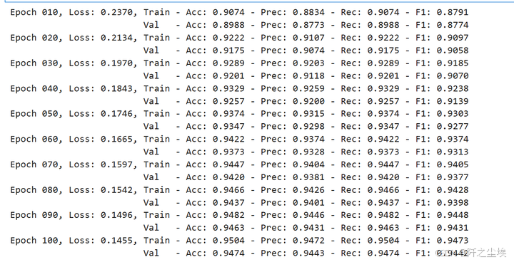
test_metrics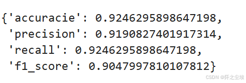
可以看到准确率和F1等评价指标都有90%以上,还是很不错的。
评估
# 评估
model.eval()
with torch.no_grad():
    test_metrics = evaluate(model, data, data.test_mask)
    test_acc = test_metrics.get('accuracie')
    test_prec = test_metrics.get('precision')
    test_rec = test_metrics.get('recall')
    test_f1 = test_metrics.get('f1_score')

    print(f'Test Acc: {test_acc:.4f} - Prec: {test_prec:.4f} - Rec: {test_rec:.4f} - F1: {test_f1:.4f}')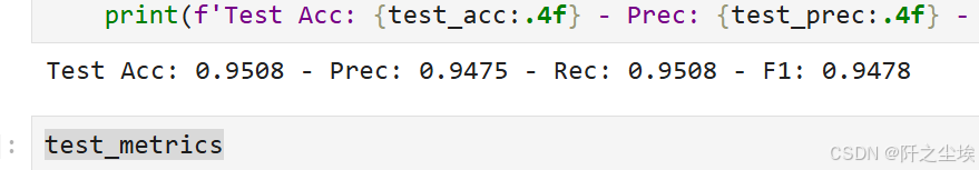
画图查看
plot_train_val_test_metrics(train_val_metrics, test_metrics, NUM_EPOCHS)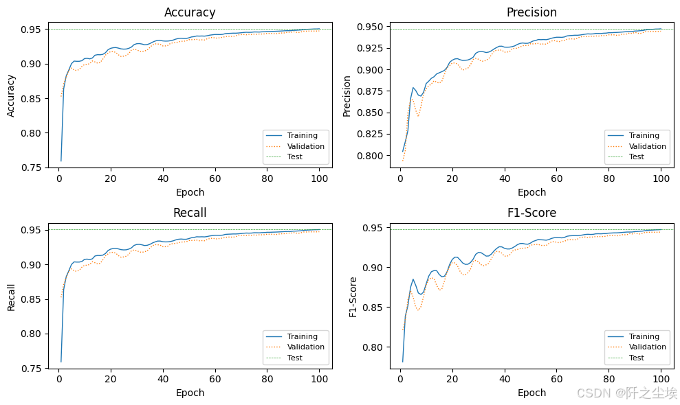
预测
train_pred = predict(model, data)[data.train_mask]
test_pred = predict(model, data)[data.test_mask]
画混淆矩阵
# --- 混淆矩阵---
print("Classification Report")
print("=====================\n")

# Train.
y_true_train = data.y[data.train_mask].cpu().numpy()
y_pred_train = train_pred.cpu().numpy()

report_train = classification_report(y_true_train, y_pred_train, target_names=mapped_classes)

print(f"{4*' '}TRAIN")
print("---------")
print(report_train)

# Test.
y_true_test = data.y[data.test_mask].cpu().numpy()
y_pred_test = test_pred.cpu().numpy()

report_test = classification_report(y_true_test, y_pred_test, target_names=mapped_classes)

print(f"{4*' '}TEST")
print("--------")
print(report_test)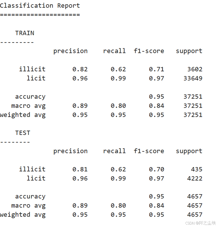
mapped_classes = np.array(['illicit', 'licit'])

# --- Confusion matrix ---
cm = confusion_matrix(data.y[data.test_mask].cpu(), test_pred.cpu())

fig, ax = plt.subplots(figsize=(6, 4))

sns.heatmap(cm, annot=True, fmt='g', cmap=plt.cm.Greens,
            annot_kws={'size': 15},
            xticklabels=mapped_classes,
            yticklabels=mapped_classes,
            linecolor='black', linewidth=0.5,
            ax=ax)
plt.xlabel('Predicted Class')
plt.ylabel('Actual Class')

# Annotate each cell with the percentage of that row.
cm_normalized = cm.astype('float') / cm.sum(axis=1)[:, np.newaxis]
for i in range(cm.shape[0]):
    for j in range(cm.shape[1]):
        count = cm[i, j]
        percentage = cm_normalized[i, j] * 100
        text = f'\n({percentage:.1f}%)'
        color = 'white' if percentage > 95 else 'black'
        ax.text(j + 0.5, i + 0.6, text,
                ha='center', va='center', fontsize=10, color=color)

plt.title('Confusion Matrix (Test set)\nGraph Convolutional Network (GCN)')
plt.show()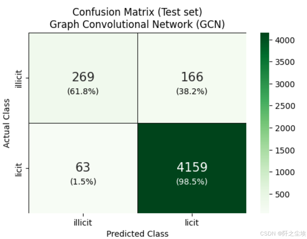
-
模型在预测未知类别方面非常出色。原因很简单,因为数据集中大部分都是未知类。
-
GCN 在预测节点是否合法方面也很出色。不过,它将 42% 的合法节点预测为未知节点。
-
该模型在预测非法节点方面表现不错,但并不确定。它只对 46% 的非法节点进行了正确分类。
train_probas = predict_probabilities(model, data)[data.train_mask]
test_probas = predict_probabilities(model, data)[data.test_mask]
train_probas_illicit = train_probas[:, 1].cpu().numpy()
train_probas_illicit
预测概率的可视化
ALPHA = 0.1

train_probas_licit = train_probas[:, 0].cpu().numpy()
train_probas_illicit = train_probas[:, 1].cpu().numpy()

test_probas_licit = test_probas[:, 0].cpu().numpy()
test_probas_illicit = test_probas[:, 1].cpu().numpy()

metrics_per_gnn['gcn']['test']['licit']['probas'] = test_probas_licit
metrics_per_gnn['gcn']['test']['illicit']['probas'] = test_probas_illicit

# -------- #
# Plotting #
# -------- #

plt.figure(figsize=(7, 4))

# Plot licit class probabilities
sns.kdeplot(train_probas_licit, fill=True, color="forestgreen", linestyle='-', alpha=ALPHA, label="Training - Licit")
sns.kdeplot(test_probas_licit, fill=True, color="green", linestyle='--', alpha=ALPHA, label="Test - Licit")

# Plot illicit class probabilities
sns.kdeplot(train_probas_illicit, fill=True, color="salmon", linestyle='-', alpha=ALPHA, label="Training - Illicit")
sns.kdeplot(test_probas_illicit, fill=True, color="red", linestyle='--', alpha=ALPHA, label="Test - Illicit")

plt.title("GCN - Predicted Probabilities")
plt.xlabel("Predicted Probability")
plt.ylabel("Density")
plt.legend(loc="upper center")

plt.show()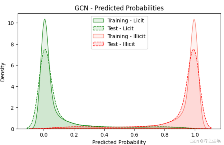
2️⃣ - GAT - Graph Attention Networks
接下来是GAT网络,注意力机制的图网络
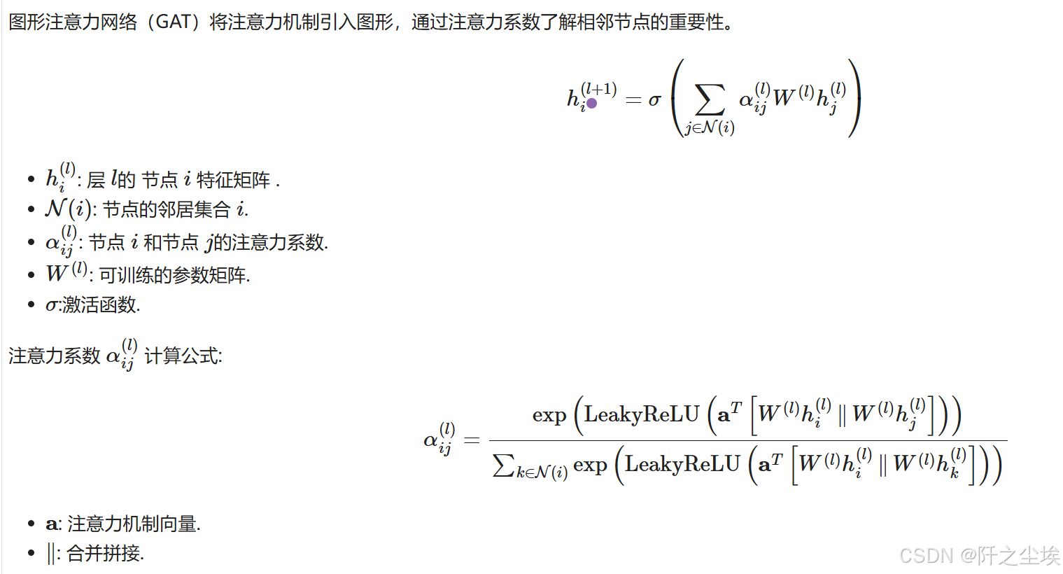
自定义类
# 定义 GAT #
class GAT(torch.nn.Module):
    def __init__(self, num_node_features, num_classes, num_heads=8):
        super(GAT, self).__init__()
        self.conv1 = GATConv(num_node_features, 8, heads=num_heads, dropout=0.6)
        self.conv2 = GATConv(8 * num_heads, num_classes, heads=1, concat=False, dropout=0.6)

    def forward(self, data):
        x, edge_index = data.x, data.edge_index
        x = self.conv1(x, edge_index)
        x = F.elu(x)
        x = self.conv2(x, edge_index)
        return F.log_softmax(x, dim=1)

# ---------- #
# Initialize #
# ---------- #

model = GAT(num_node_features=data.num_features, num_classes=len(le.classes_)).to(device)
optimizer = torch.optim.Adam(model.parameters(), lr=0.01, weight_decay=0.0005)
criterion = torch.nn.CrossEntropyLoss()  # Since we have a multiclass classification problem.

data = data.to(device)
训练,和前面一样的
# Train #
train_val_metrics = train_gnn(NUM_EPOCHS,  data,
                              model, optimizer, criterion)

metrics_per_gnn['gat']['val']['precisions'] = train_val_metrics['val']['precisions']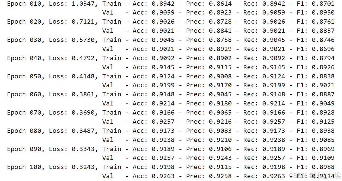
评估
# Evaluate #

model.eval()
with torch.no_grad():

    test_metrics = evaluate(model, data, data.test_mask)
    test_acc = test_metrics.get('accuracie')
    test_prec = test_metrics.get('precision')
    test_rec = test_metrics.get('recall')
    test_f1 = test_metrics.get('f1_score')

    print(f'Test Acc: {test_acc:.4f} - Prec: {test_prec:.4f} - Rec: {test_rec:.4f} - F1: {test_f1:.4f}')
plot_train_val_test_metrics(train_val_metrics, test_metrics, NUM_EPOCHS)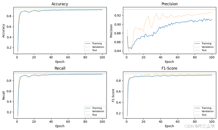
混淆矩阵
test_pred = predict(model, data)[data.test_mask]

# --- 混淆矩阵 ---
cm = confusion_matrix(data.y[data.test_mask].cpu(), test_pred.cpu())

fig, ax = plt.subplots(figsize=(6, 4))

sns.heatmap(cm, annot=True, fmt='g', cmap=plt.cm.Greens,
            annot_kws={'size': 15},
            xticklabels=mapped_classes,
            yticklabels=mapped_classes,
            linecolor='black', linewidth=0.5,
            ax=ax)
plt.xlabel('Predicted Class')
plt.ylabel('Actual Class')

# Annotate each cell with the percentage of that row.
cm_normalized = cm.astype('float') / cm.sum(axis=1)[:, np.newaxis]
for i in range(cm.shape[0]):
    for j in range(cm.shape[1]):
        count = cm[i, j]
        percentage = cm_normalized[i, j] * 100
        text = f'\n({percentage:.1f}%)'
        color = 'white' if percentage > 95 else 'black'
        ax.text(j + 0.5, i + 0.6, text,
                ha='center', va='center', fontsize=10, color=color)

plt.title('Confusion Matrix\nGraph Attention Network (GAT)')
plt.show()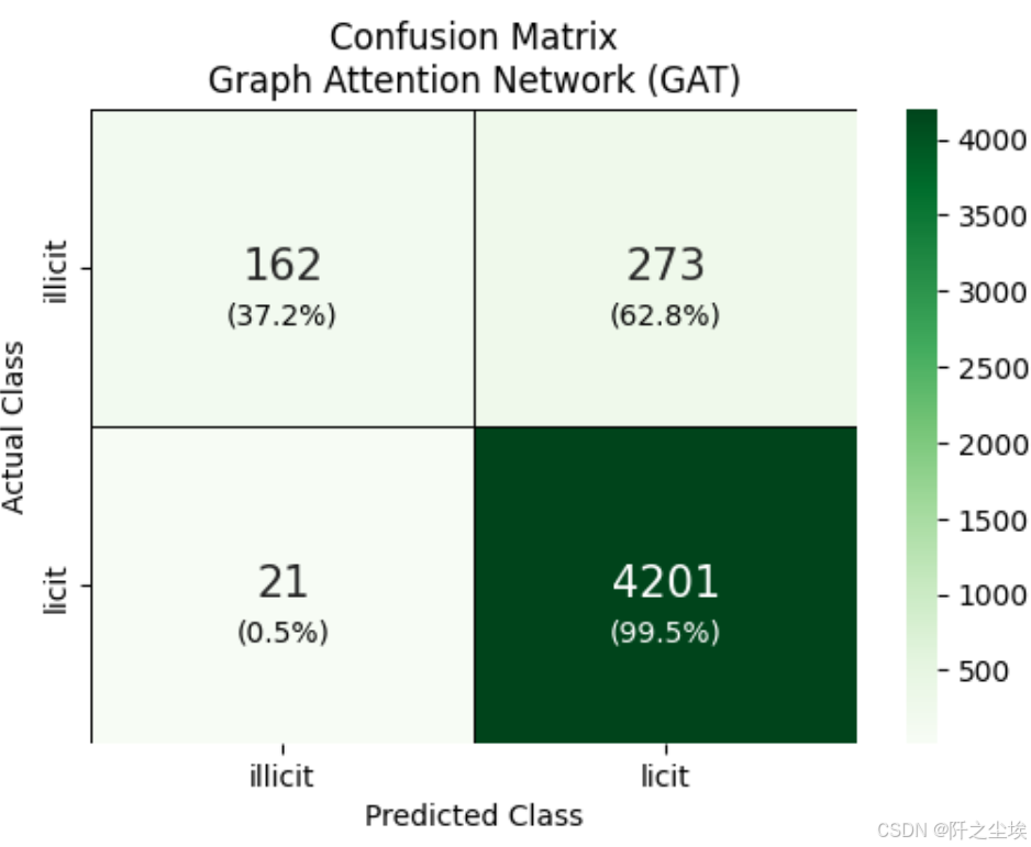
train_probas = predict_probabilities(model, data)[data.train_mask]
test_probas = predict_probabilities(model, data)[data.test_mask]
train_probas_illicit = train_probas[:, 1].cpu().numpy()
train_probas_illicit
预测概率可视化
ALPHA = 0.1

train_probas_licit = train_probas[:, 0].cpu().numpy()
train_probas_illicit = train_probas[:, 1].cpu().numpy()

test_probas_licit = test_probas[:, 0].cpu().numpy()
test_probas_illicit = test_probas[:, 1].cpu().numpy()

metrics_per_gnn['gat']['test']['licit']['probas'] = test_probas_licit
metrics_per_gnn['gat']['test']['illicit']['probas'] = test_probas_illicit

# Plotting #

plt.figure(figsize=(7, 4))

# Plot licit class probabilities
sns.kdeplot(train_probas_licit, fill=True, color="forestgreen", linestyle='-', alpha=ALPHA, label="Training - Licit")
sns.kdeplot(test_probas_licit, fill=True, color="green", linestyle='--', alpha=ALPHA, label="Test - Licit")

# Plot illicit class probabilities
sns.kdeplot(train_probas_illicit, fill=True, color="salmon", linestyle='-', alpha=ALPHA, label="Training - Illicit")
sns.kdeplot(test_probas_illicit, fill=True, color="red", linestyle='--', alpha=ALPHA, label="Test - Illicit")

plt.title("GAT - Predicted Probabilities")
plt.xlabel("Predicted Probability")
plt.ylabel("Density")
plt.legend(loc="upper center")

plt.show()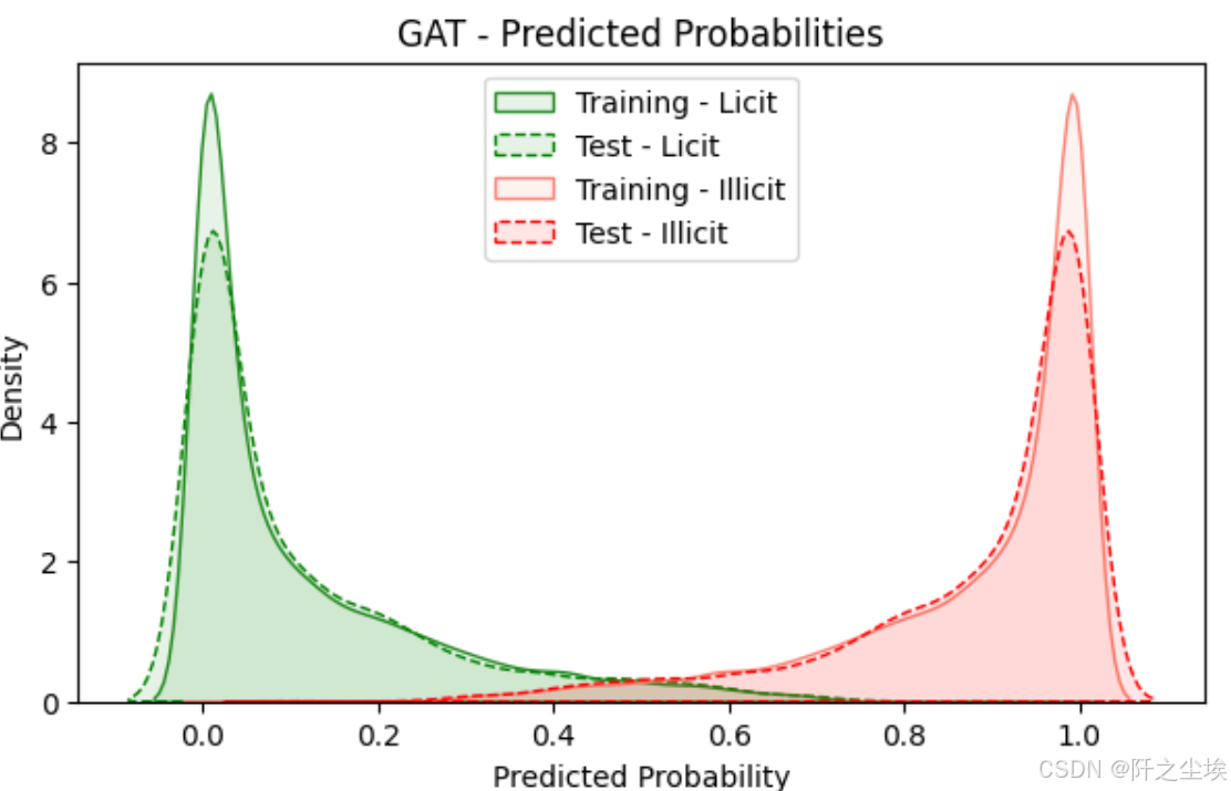
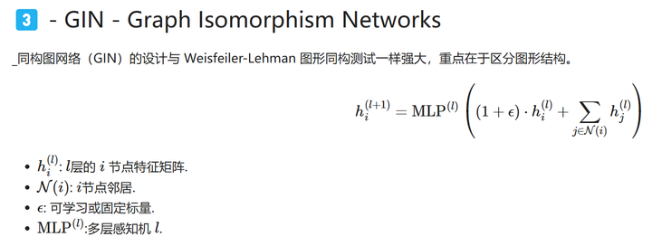
3️⃣ - GIN - Graph Isomorphism Networks
下面是GIN网络。 汇集相邻节点的特征,然后应用 MLP 生成下一层的节点特征。 加入ϵ可以区分节点及其邻居
自定义网络
# 定义 GIN #
from torch_geometric.nn import GINConv, global_add_pool
import torch.nn.functional as F

class GIN(torch.nn.Module):
    def __init__(self, num_node_features, num_classes):
        super(GIN, self).__init__()

        # 1st GIN layer.
        nn1 = torch.nn.Sequential(
            torch.nn.Linear(num_node_features, 64),
            torch.nn.ReLU(),
            torch.nn.Linear(64, 64)
        )
        self.conv1 = GINConv(nn1)

        # 2nd GIN layer.
        nn2 = torch.nn.Sequential(
            torch.nn.Linear(64, 64),
            torch.nn.ReLU(),
            torch.nn.Linear(64, 64)
        )
        self.conv2 = GINConv(nn2)
        self.fc = torch.nn.Linear(64, num_classes)

    def forward(self, data):
        x, edge_index, batch = data.x, data.edge_index, data.batch

        x = self.conv1(x, edge_index)
        x = F.relu(x)
        x = self.conv2(x, edge_index)
#         x = global_add_pool(x, batch)
        x = self.fc(x)

        return F.log_softmax(x, dim=1)

# 初始化 #

model = GIN(num_node_features=data.num_features, num_classes=len(le.classes_)).to(device)
optimizer = torch.optim.Adam(model.parameters(), lr=0.01, weight_decay=0.0005)
criterion = torch.nn.CrossEntropyLoss()

# # Handle the class imbalance
# class_counts = torch.bincount(data.y)
# class_weights = 1. / class_counts.float()
# criterion = torch.nn.CrossEntropyLoss(weight=class_weights)

data = data.to(device)
训练
# 训练 #

train_val_metrics = train_gnn(NUM_EPOCHS,  data,
                              model, optimizer, criterion)

metrics_per_gnn['gin']['val']['precisions'] = train_val_metrics['val']['precisions']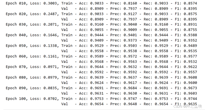
这个看目前打印的数值感觉效果比前两个好。
评估
model.eval()
with torch.no_grad():

    test_metrics = evaluate(model, data, data.test_mask)
    test_acc = test_metrics.get('accuracie')
    test_prec = test_metrics.get('precision')
    test_rec = test_metrics.get('recall')
    test_f1 = test_metrics.get('f1_score')

    print(f'Test Acc: {test_acc:.4f} - Prec: {test_prec:.4f} - Rec: {test_rec:.4f} - F1: {test_f1:.4f}')
可视化
plot_train_val_test_metrics(train_val_metrics, test_metrics, NUM_EPOCHS)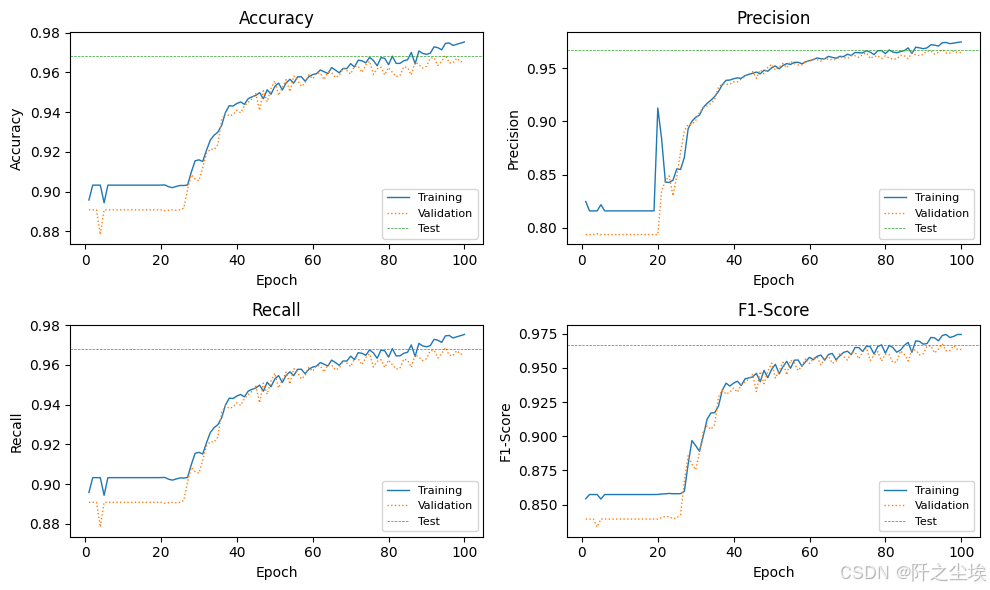
混淆矩阵
test_pred = predict(model, data)[data.test_mask]

# --- 混淆矩阵 ---
cm = confusion_matrix(data.y[data.test_mask].cpu(), test_pred.cpu())

fig, ax = plt.subplots(figsize=(6, 4))

sns.heatmap(cm, annot=True, fmt='g', cmap=plt.cm.Greens,
            annot_kws={'size': 15},
            xticklabels=mapped_classes,
            yticklabels=mapped_classes,
            linecolor='black', linewidth=0.5,
            ax=ax)
plt.xlabel('Predicted Class')
plt.ylabel('Actual Class')

# Annotate each cell with the percentage of that row.
cm_normalized = cm.astype('float') / cm.sum(axis=1)[:, np.newaxis]
for i in range(cm.shape[0]):
    for j in range(cm.shape[1]):
        count = cm[i, j]
        percentage = cm_normalized[i, j] * 100
        text = f'\n({percentage:.1f}%)'
        color = 'white' if percentage > 95 else 'black'
        ax.text(j + 0.5, i + 0.6, text,
                ha='center', va='center', fontsize=10, color=color)

plt.title('Confusion Matrix\nGraph Isomorphism Network (GIN)')
plt.show()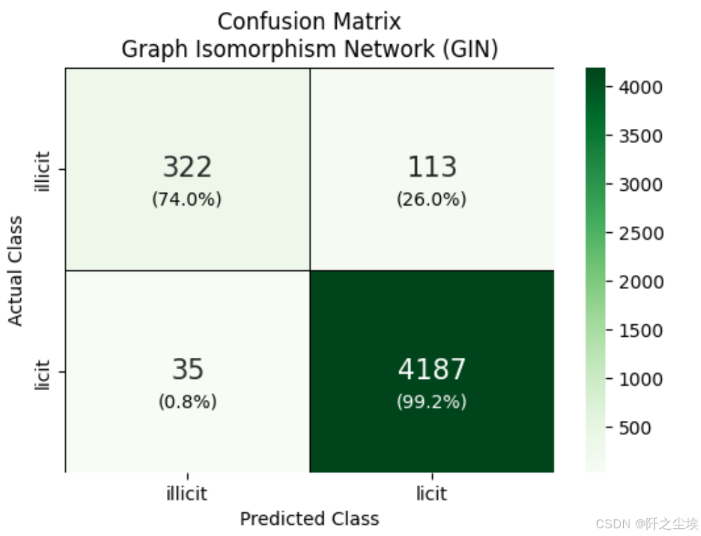
train_probas = predict_probabilities(model, data)[data.train_mask]
test_probas = predict_probabilities(model, data)[data.test_mask]
train_probas_illicit = train_probas[:, 1].cpu().numpy()
train_probas_illicit
预测概率可视化
ALPHA = 0.1

train_probas_licit = train_probas[:, 0].cpu().numpy()
train_probas_illicit = train_probas[:, 1].cpu().numpy()

test_probas_licit = test_probas[:, 0].cpu().numpy()
test_probas_illicit = test_probas[:, 1].cpu().numpy()

metrics_per_gnn['gin']['test']['licit']['probas'] = test_probas_licit
metrics_per_gnn['gin']['test']['illicit']['probas'] = test_probas_illicit

# Plotting #

plt.figure(figsize=(7, 4))

# Plot licit class probabilities
sns.kdeplot(train_probas_licit, fill=True, color="forestgreen", linestyle='-', alpha=ALPHA, label="Training - Licit")
sns.kdeplot(test_probas_licit, fill=True, color="green", linestyle='--', alpha=ALPHA, label="Test - Licit")

# Plot illicit class probabilities
sns.kdeplot(train_probas_illicit, fill=True, color="salmon", linestyle='-', alpha=ALPHA, label="Training - Illicit")
sns.kdeplot(test_probas_illicit, fill=True, color="red", linestyle='--', alpha=ALPHA, label="Test - Illicit")

plt.title("GIN - Predicted Probabilities")
plt.xlabel("Predicted Probability")
plt.ylabel("Density")
plt.legend(loc="upper center")

plt.show()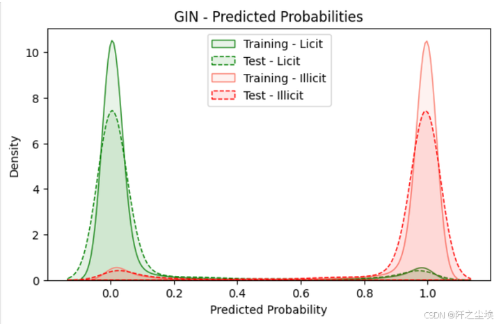
⚖️ GNNs 对比
下面把三个图神经网络的效果都进行一下对比
plt.figure(figsize=(8, 4),dpi=128)

epochs = range(1, len(metrics_per_gnn['gcn']['val']['precisions']) + 1)

plt.plot(epochs, metrics_per_gnn['gcn']['val']['precisions'], color='C0', linewidth=1.2, linestyle='--', label='GCN')
plt.plot(epochs, metrics_per_gnn['gat']['val']['precisions'], color='C1', linewidth=1.2, linestyle='-.', label='GAT')
plt.plot(epochs, metrics_per_gnn['gin']['val']['precisions'], color='C2', linewidth=1.2, linestyle=':', label='GIN')

plt.xlabel('Epoch')
plt.ylabel('Precision')
plt.title('Validation Precisions Comparison Across GNN Models')
plt.legend(fontsize=10)
plt.grid(False)
plt.tight_layout()
plt.show()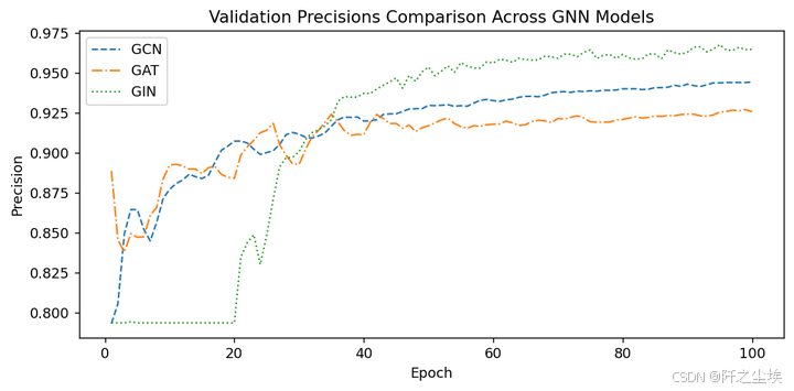
就看精准度的话应该是gin网络是最好的。精度而言,GIN 的总体表现似乎最好,尤其是在后期稳定之后。它的精度最高,但初期表现出不稳定性。
概率对比
ALPHA = 0.9   ;   FILL = False

plt.figure(figsize=(8, 5),dpi=128)

sns.kdeplot(metrics_per_gnn['gcn']['test']['licit']['probas'], fill=FILL, color="forestgreen", linestyle='-', alpha=ALPHA, label="GCN - Licit")
sns.kdeplot(metrics_per_gnn['gcn']['test']['illicit']['probas'], fill=FILL, color="salmon", linestyle='-', alpha=ALPHA, label="GCN - Illicit")

sns.kdeplot(metrics_per_gnn['gat']['test']['licit']['probas'], fill=FILL, color="darkgreen", linestyle='--', alpha=ALPHA, label="GAT - Licit")
sns.kdeplot(metrics_per_gnn['gat']['test']['illicit']['probas'], fill=FILL, color="red", linestyle='--', alpha=ALPHA, label="GAT - Illicit")

sns.kdeplot(metrics_per_gnn['gin']['test']['licit']['probas'], fill=FILL, color="lightgreen", linestyle=':', alpha=ALPHA, label="GIN - Licit")
sns.kdeplot(metrics_per_gnn['gin']['test']['illicit']['probas'], fill=FILL, color="darkred", linestyle=':', alpha=ALPHA, label="GIN - Illicit")

plt.title("Predicted Probabilities Comparison Across GNN Models")
plt.xlabel("Predicted Probability")
plt.ylabel("Density")
plt.legend(loc="upper center", ncol=2)  # bbox_to_anchor=(0.5, -0.1),
plt.tight_layout()

plt.show()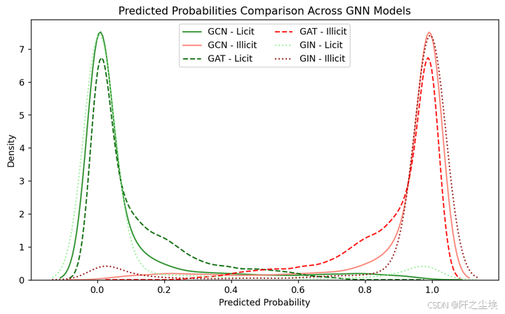
可以清楚的看到每种网络它各自预测的分布,以及正确与否的对比。
data_temp = []

for model in ['gcn', 'gat', 'gin']:
    for category in ['licit', 'illicit']:
        probas = metrics_per_gnn[model]['test'][category]['probas']
        data_temp.extend([(model.upper(), category.capitalize(), proba) for proba in probas])

temp = pd.DataFrame(data_temp, columns=['Model', 'Class', 'Probability'])

plt.figure(figsize=(8, 4),dpi=128)

flierprops = dict(marker='o', markerfacecolor='None', markersize=5,  markeredgecolor='C0', alpha=0.2)

ax = sns.boxplot(y='Model', x='Probability', hue='Class', data=temp,
                 linewidth=2.5,
                 fliersize=0.5,
                 palette={
                     'Licit': 'forestgreen',
                     'Illicit': 'indianred'
                 },
                 flierprops=flierprops
)


plt.grid(True, which='both', axis='x', color='lightgrey', linestyle='-', linewidth=0.5)
plt.title("Comparison of Predicted Probabilities Across GNN's")
plt.xlabel("Predicted Probability")
plt.ylabel("GNN Model")
plt.legend(loc="center left", bbox_to_anchor=(1, 0.5), ncol=1)
plt.tight_layout()
plt.show()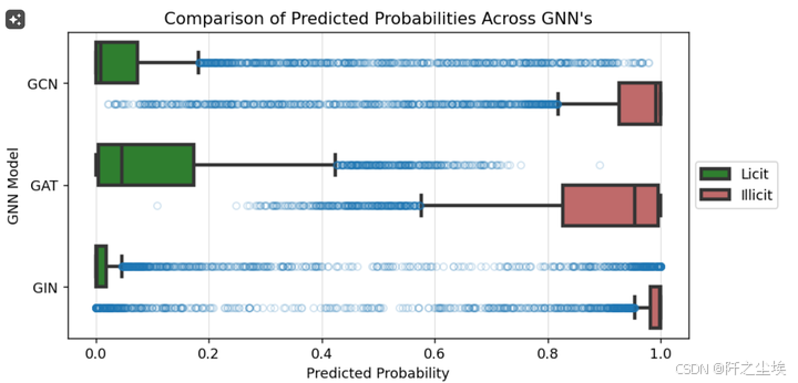
可以看到gin的箱体是最小的,它的预测的数据也是最为稳定的。效果也是最好的。
# 用 t 检验来比较 # # 每个模型中合法与非法预测的平均值 #
comparisons = [('gcn', 'gat'), ('gcn', 'gin'), ('gat', 'gin')]
results = []

for model1, model2 in comparisons:
    for category in ['licit', 'illicit']:
        probas1 = metrics_per_gnn[model1]['test'][category]['probas']
        probas2 = metrics_per_gnn[model2]['test'][category]['probas']
        t_stat, p_val = ttest_ind(probas1, probas2, equal_var=False)
        if p_val < 0.05:
            results.append(f"Significant difference between {model1.upper()} and {model2.upper()} for {category.capitalize()} predictions (p-value: {p_val:.4f})")

for result in results:
    print(result)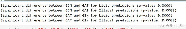
p为0.00,表示都是显著的,说明模型里面合法跟非法的这个平均值有显著性差异。
对比一下他们模型预测结果的相关性
combinations = [('GCN', 'GAT'), ('GCN', 'GIN'), ('GAT', 'GIN')]

fig, axes = plt.subplots(1, 3, figsize=(15, 4),dpi=128)

for ax, (model1, model2) in zip(axes, combinations):
    scatter_data = pd.DataFrame({
        f'{model1}_Probabilities': temp[temp['Model'] == model1]['Probability'].values,
        f'{model2}_Probabilities': temp[temp['Model'] == model2]['Probability'].values   })

    sns.scatterplot(data=scatter_data,
        x=f'{model1}_Probabilities',y=f'{model2}_Probabilities',
        color='C0',    edgecolor='white',marker='o',         alpha=0.3, ax=ax )

    corr_value = np.corrcoef(temp[temp['Model'] == model1]['Probability'],
                             temp[temp['Model'] == model2]['Probability'])[0, 1]

    ax.plot([0, 1], [0, 1], ls='--', color='lightcoral', label=f'Perfect Correlation', alpha=1.0)

    ax.set_title(f'{model1} vs {model2}\nCorr: {corr_value:.3f}')
    ax.set_xlabel(f'{model1} Probabilities')
    ax.set_ylabel(f'{model2} Probabilities')
    ax.legend(loc='upper left')

plt.tight_layout()
plt.show()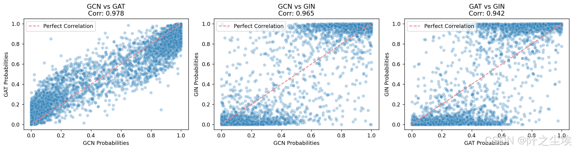
三者的情况都是类似的,相关性都很高,但综合来看的话,在这个案例上还是gin的效果是最好的,gcn其次。gat表现效果最差,可能由于他注意力机制主要用于设计时间序列的吧,对这个数据不是很适用。
后续改进想法
-
将每个 GNN 使用的代码外包给全局方法。这将使笔记本更简短、更易读。
-
只在已知节点上进行训练。然后在一小部分未训练过的已知节点上进行验证。然后对未知节点进行预测。
-
为每种 GNN 类型添加简短解释和公式。
-
开发一个基线模型(非 GNN)。
-
执行一些图形可解释性方法,例如 GNNExplainer。
-
对不同大小的节点特征及其对性能的影响进行分析。
看到这基本上最简单的图神经网络的数据结构以及训练使用方法应该都明了了。后面可以再进行更复杂的任务学习。本案例全部数据和代码在:图神经网络
创作不易,看官觉得写得还不错的话点个关注和赞吧,本人会持续更新python数据分析领域的代码文章~(需要定制类似的代码可私信)