调制信号识别系列 (一):基准模型
说明:本文包含对CNN和CNN+LSTM基准模型的复现,模型架构参考下述两篇文章
文章目录
- 调制信号识别系列 (一):基准模型
- 一、论文
- 1、DL-PR: Generalized automatic modulation classification method based on deep learning with priori regularization
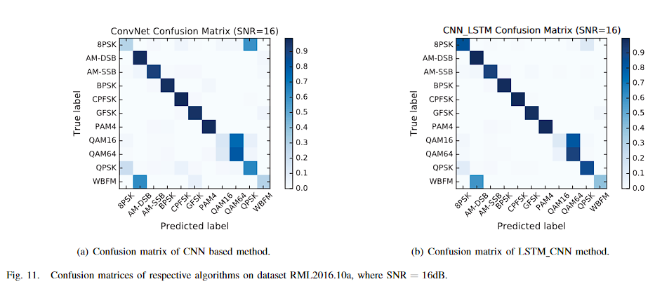
- 2、A Deep Learning Approach for Modulation Recognition via Exploiting Temporal Correlations
- 二、流程
- 1、数据加载
- 2、训练测试
- 3、可视化
- 三、模型
- 1、CNN
- 2、CNN+LSTM(DL-PR)
- 3、CNN+LSTM
- 四、对比
- 1、论文1
- 2、论文2
- 五、总结
一、论文
1、DL-PR: Generalized automatic modulation classification method based on deep learning with priori regularization
- https://www.sciencedirect.com/science/article/pii/S095219762300266X

2、A Deep Learning Approach for Modulation Recognition via Exploiting Temporal Correlations
-
2018 IEEE 19th International Workshop on Signal Processing Advances in Wireless Communications (SPAWC)
-
https://ieeexplore.ieee.org/abstract/document/8445938
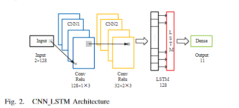
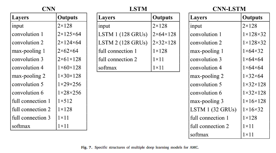
Note that before each convolutional layer, we use the zero-padding method to control the spatial size of the output volumes. Specifically, we pad the input volume with two zeros around the border, thus the output volume of the second convolutional layer is of size 32 × 132. We then take 32 as the dimensionality of the input and 132 as the time steps in LSTM layer. Dropout method is also used to prevent the neural network from overfitting. Compared to architecture in [12], we can see that we replace the third dense fully-connected layer with a LSTM layer. Our simulations suggest that this replacement not only reduces the number of parameters by an order of magnitude, but also leads to a significant performance improvement.
请注意,在每个卷积层之前,我们使用零填充方法来控制输出卷的空间大小。具体来说,我们在输入量的边界周围填充两个零,因此第二个卷积层的输出量的大小为 32 × 132。然后我们将 32 作为输入的维度,将 132 作为 LSTM 层的时间步长。 Dropout方法也用于防止神经网络过拟合。与[12]中的架构相比,我们可以看到我们用 LSTM 层替换了第三个密集全连接层。我们的模拟表明,这种替换不仅将参数数量减少了一个数量级,而且还带来了显着的性能改进。
二、流程
1、数据加载
import torch
import torch.nn as nn
import torch.optim as optim
from torch.utils.data import DataLoader, TensorDataset, random_split
import pandas as pd
import numpy as np
import matplotlib.pyplot as plt
from sklearn.metrics import confusion_matrix, ConfusionMatrixDisplay
from torchsummary import summary
# 加载数据
csv_file_path = 'snr_data/output_data_snr_6.csv'
data_frame = pd.read_csv(csv_file_path)

# 提取前256列数据并转换为张量
vectors = torch.tensor(data_frame.iloc[:, :256].values, dtype=torch.float32)

# 将256维向量转换为2x128的矩阵形式
vectors = vectors.view(-1, 2, 128)

# 划分训练集和测试集索引
train_size = int(0.8 * len(vectors))
test_size = len(vectors) - train_size
train_indices, test_indices = random_split(range(len(vectors)), [train_size, test_size])

# 使用训练集的统计量进行归一化
train_vectors = vectors[train_indices]

# 对IQ分量分别进行归一化
train_mean_I = train_vectors[:, 0, :].mean(dim=0, keepdim=True)
train_std_I = train_vectors[:, 0, :].std(dim=0, keepdim=True)

train_mean_Q = train_vectors[:, 1, :].mean(dim=0, keepdim=True)
train_std_Q = train_vectors[:, 1, :].std(dim=0, keepdim=True)

# 归一化整个数据集
vectors[:, 0, :] = (vectors[:, 0, :] - train_mean_I) / train_std_I
vectors[:, 1, :] = (vectors[:, 1, :] - train_mean_Q) / train_std_Q

# 提取Mod_Type列并转换为数值标签
mod_types = data_frame['Mod_Type'].astype('category').cat.codes.values
labels = torch.tensor(mod_types, dtype=torch.long)

# 创建TensorDataset
dataset = TensorDataset(vectors, labels)

# 创建训练集和测试集
train_dataset = TensorDataset(vectors[train_indices], labels[train_indices])
test_dataset = TensorDataset(vectors[test_indices], labels[test_indices])

# 创建DataLoader
train_loader = DataLoader(train_dataset, batch_size=32, shuffle=True)
test_loader = DataLoader(test_dataset, batch_size=32, shuffle=False)
# 替换模型架构
2、训练测试
criterion = nn.CrossEntropyLoss()
optimizer = optim.Adam(model.parameters(), lr=0.001)
num_epochs = 50
train_losses = []
test_losses = []
train_accuracies = []
test_accuracies = []
def calculate_accuracy(outputs, labels):
_, predicted = torch.max(outputs, 1)
total = labels.size(0)
correct = (predicted == labels).sum().item()
return correct / total
for epoch in range(num_epochs):
# 训练阶段
model.train()
running_loss = 0.0
correct = 0
total = 0
for inputs, labels in train_loader:
inputs = inputs.to(device)
labels = labels.to(device)
optimizer.zero_grad()
outputs = model(inputs)
loss = criterion(outputs, labels)
loss.backward()
optimizer.step()
running_loss += loss.item()
correct += (outputs.argmax(1) == labels).sum().item()
total += labels.size(0)
train_loss = running_loss / len(train_loader)
train_accuracy = correct / total
train_losses.append(train_loss)
train_accuracies.append(train_accuracy)
# 测试阶段
model.eval()
running_loss = 0.0
correct = 0
total = 0
with torch.no_grad():
for inputs, labels in test_loader:
inputs = inputs.to(device)
labels = labels.to(device)
outputs = model(inputs)
loss = criterion(outputs, labels)
running_loss += loss.item()
correct += (outputs.argmax(1) == labels).sum().item()
total += labels.size(0)
test_loss = running_loss / len(test_loader)
test_accuracy = correct / total
test_losses.append(test_loss)
test_accuracies.append(test_accuracy)
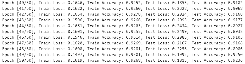
print(f"Epoch [{epoch+1}/{num_epochs}], Train Loss: {train_loss:.4f}, Train Accuracy: {train_accuracy:.4f}, Test Loss: {test_loss:.4f}, Test Accuracy: {test_accuracy:.4f}")
print("Training complete.")
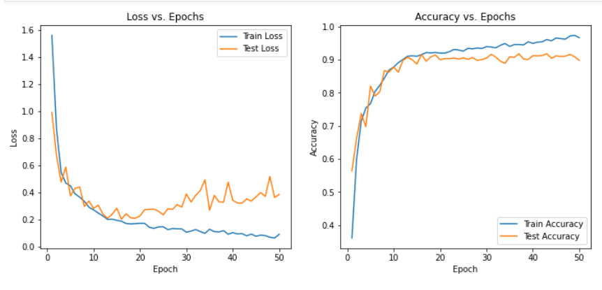
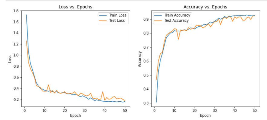
3、可视化
epochs = range(1, num_epochs + 1)

plt.figure(figsize=(12, 5))

# 绘制损失图像
plt.subplot(1, 2, 1)
plt.plot(epochs, train_losses, label='Train Loss')
plt.plot(epochs, test_losses, label='Test Loss')
plt.xlabel('Epoch')
plt.ylabel('Loss')
plt.legend()
plt.title('Loss vs. Epochs')

# 绘制准确率图像
plt.subplot(1, 2, 2)
plt.plot(epochs, train_accuracies, label='Train Accuracy')
plt.plot(epochs, test_accuracies, label='Test Accuracy')
plt.xlabel('Epoch')
plt.ylabel('Accuracy')
plt.legend()
plt.title('Accuracy vs. Epochs')

plt.show()
三、模型
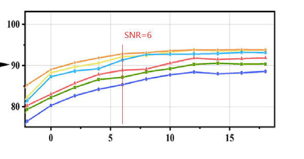
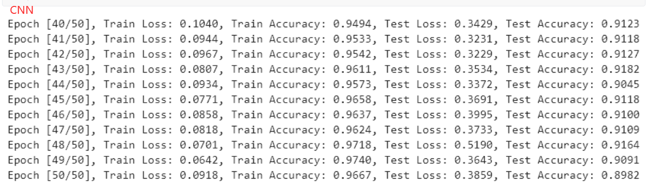
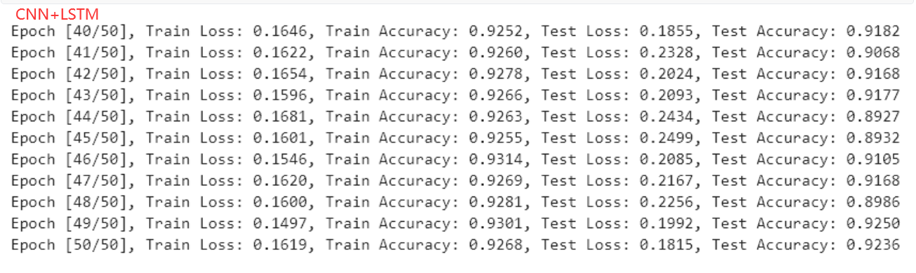
说明:下述模型均在SNR=6dB RadioML2016.10a数据集下的实验结果,仅使用原始的IQ分量信息,未使用数据增强,也未进行调参
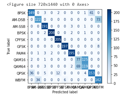
1、CNN
class CNNModel(nn.Module):
    def __init__(self):
        super(CNNModel, self).__init__()
        self.conv1 = nn.Conv2d(1, 64, (1, 4), stride=1)
        self.conv2 = nn.Conv2d(64, 64, (1, 2), stride=1)
        self.pool1 = nn.MaxPool2d((1, 2))
        self.conv3 = nn.Conv2d(64, 128, (1, 2), stride=1)
        self.conv4 = nn.Conv2d(128, 128, (2, 2), stride=1)
        self.pool2 = nn.MaxPool2d((1, 2))
        self.conv5 = nn.Conv2d(128, 256, (1, 2), stride=1)
        self.conv6 = nn.Conv2d(256, 256, (1, 2), stride=1)
        self.fc1 = nn.Linear(256 * 1 * 28, 512)
        self.fc2 = nn.Linear(512, 128)
        self.fc3 = nn.Linear(128, 11)

    def forward(self, x):
        x = x.unsqueeze(1)  # 添加通道维度
        x = torch.relu(self.conv1(x))
        x = torch.relu(self.conv2(x))
        x = self.pool1(x)
        x = torch.relu(self.conv3(x))
        x = torch.relu(self.conv4(x))
        x = self.pool2(x)
        x = torch.relu(self.conv5(x))
        x = torch.relu(self.conv6(x))
        x = x.view(x.size(0), -1)
        x = torch.relu(self.fc1(x))
        x = torch.relu(self.fc2(x))
        x = self.fc3(x)
        return x

model = CNNModel()
summary(model, (2, 128))

----------------------------------------------------------------
        Layer (type)               Output Shape         Param #
================================================================
            Conv2d-1           [-1, 64, 2, 125]             320
            Conv2d-2           [-1, 64, 2, 124]           8,256
         MaxPool2d-3            [-1, 64, 2, 62]               0
            Conv2d-4           [-1, 128, 2, 61]          16,512
            Conv2d-5           [-1, 128, 1, 60]          65,664
         MaxPool2d-6           [-1, 128, 1, 30]               0
            Conv2d-7           [-1, 256, 1, 29]          65,792
            Conv2d-8           [-1, 256, 1, 28]         131,328
            Linear-9                  [-1, 512]       3,670,528
           Linear-10                  [-1, 128]          65,664
           Linear-11                   [-1, 11]           1,419
================================================================
Total params: 4,025,483
Trainable params: 4,025,483
Non-trainable params: 0
----------------------------------------------------------------
Input size (MB): 0.00
Forward/backward pass size (MB): 0.63
Params size (MB): 15.36
Estimated Total Size (MB): 15.98
2、CNN+LSTM(DL-PR)
import torch
import torch.nn as nn

class CNNLSTMModel(nn.Module):
    def __init__(self):
        super(CNNLSTMModel, self).__init__()
        self.conv1 = nn.Conv2d(1, 32, (2, 3), stride=1, padding=(0,1))  # Adjusted input channels and filters
        self.conv2 = nn.Conv2d(32, 32, (1, 3), stride=1, padding=(0,1))
        self.pool1 = nn.MaxPool2d((1, 2))
        self.conv3 = nn.Conv2d(32, 64, (1, 3), stride=1, padding=(0,1))
        self.conv4 = nn.Conv2d(64, 64, (1, 3), stride=1, padding=(0,1))
        self.pool2 = nn.MaxPool2d((1, 2))
        self.conv5 = nn.Conv2d(64, 128, (1, 3), stride=1, padding=(0,1))
        self.conv6 = nn.Conv2d(128, 128, (1, 3), stride=1, padding=(0,1))
        self.pool3 = nn.MaxPool2d((1, 2))

        self.lstm = nn.LSTM(128, 32, batch_first=True)  # Adjusted input size and LSTM hidden size
        self.fc1 = nn.Linear(32, 128)
        self.fc2 = nn.Linear(128, 11)

    def forward(self, x):
        #print("x:",x.shape)
        if x.dim() == 3:
            x = x.unsqueeze(1)  # 假设x的形状是[2, 128], 这将改变它为[1, 2, 128]
        #print("x.unsqueeze(0):",x.shape)
        x = torch.relu(self.conv1(x))
        x = torch.relu(self.conv2(x))
        x = self.pool1(x)
        x = torch.relu(self.conv3(x))
        x = torch.relu(self.conv4(x))
        x = self.pool2(x)
        x = torch.relu(self.conv5(x))
        x = torch.relu(self.conv6(x))
        x = self.pool3(x)

        # Prepare input for LSTM
        x = x.view(x.size(0), 16, 128)  # Adjusted view
        #print(x.shape)
        x, (hn, cn) = self.lstm(x)
        x = x[:, -1, :]  # Get the last output of the LSTM

        x = torch.relu(self.fc1(x))
        x = self.fc2(x)
        return x

model = CNNLSTMModel()
summary(model,input_size=(1, 2, 128))

==========================================================================================
Layer (type:depth-idx)                   Output Shape              Param #
==========================================================================================
CNNLSTMModel                             [1, 11]                   --
├─Conv2d: 1-1                            [1, 32, 1, 128]           224
├─Conv2d: 1-2                            [1, 32, 1, 128]           3,104
├─MaxPool2d: 1-3                         [1, 32, 1, 64]            --
├─Conv2d: 1-4                            [1, 64, 1, 64]            6,208
├─Conv2d: 1-5                            [1, 64, 1, 64]            12,352
├─MaxPool2d: 1-6                         [1, 64, 1, 32]            --
├─Conv2d: 1-7                            [1, 128, 1, 32]           24,704
├─Conv2d: 1-8                            [1, 128, 1, 32]           49,280
├─MaxPool2d: 1-9                         [1, 128, 1, 16]           --
├─LSTM: 1-10                             [1, 16, 32]               20,736
├─Linear: 1-11                           [1, 128]                  4,224
├─Linear: 1-12                           [1, 11]                   1,419
==========================================================================================
Total params: 122,251
Trainable params: 122,251
Non-trainable params: 0
Total mult-adds (M): 4.32
==========================================================================================
Input size (MB): 0.00
Forward/backward pass size (MB): 0.20
Params size (MB): 0.49
Estimated Total Size (MB): 0.69
==========================================================================================
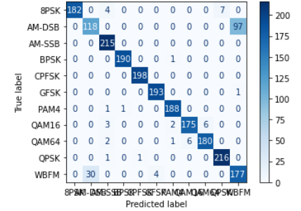
3、CNN+LSTM
# 定义结合CNN和LSTM的模型
class CNNLSTMModel(nn.Module):
    def __init__(self):
        super(CNNLSTMModel, self).__init__()
        self.conv1 = nn.Conv2d(1, 64, (1, 4), stride=1)
        self.conv2 = nn.Conv2d(64, 64, (1, 2), stride=1)
        self.pool1 = nn.MaxPool2d((1, 2))
        self.conv3 = nn.Conv2d(64, 128, (1, 2), stride=1)
        self.conv4 = nn.Conv2d(128, 128, (2, 2), stride=1)
        self.pool2 = nn.MaxPool2d((1, 2))
        self.conv5 = nn.Conv2d(128, 256, (1, 2), stride=1)
        self.conv6 = nn.Conv2d(256, 256, (1, 2), stride=1)

        self.lstm = nn.LSTM(256, 128, batch_first=True)

        self.fc1 = nn.Linear(128, 512)
        self.fc2 = nn.Linear(512, 128)
        self.fc3 = nn.Linear(128, 11)

    def forward(self, x):
        x = x.unsqueeze(1)  # 添加通道维度
        x = torch.relu(self.conv1(x))
        x = torch.relu(self.conv2(x))
        x = self.pool1(x)
        x = torch.relu(self.conv3(x))
        x = torch.relu(self.conv4(x))
        x = self.pool2(x)
        x = torch.relu(self.conv5(x))
        x = torch.relu(self.conv6(x))

        # 重新调整x的形状以适应LSTM
        x = x.squeeze(2).permute(0, 2, 1)  # 变为(batch_size, 128, 256)

        # 通过LSTM
        x, _ = self.lstm(x)

        # 取最后一个时间步的输出
        x = x[:, -1, :]

        # 全连接层
        x = torch.relu(self.fc1(x))
        x = torch.relu(self.fc2(x))
        x = self.fc3(x)
        return x
device = torch.device('cuda' if torch.cuda.is_available() else 'cpu')
model = CNNLSTMModel().to(device)
summary(model,input_size=(1, 2, 128))
==========================================================================================
Layer (type:depth-idx)                   Output Shape              Param #
==========================================================================================
CNNLSTMModel                             [1, 11]                   --
├─Conv2d: 1-1                            [1, 64, 2, 125]           320
├─Conv2d: 1-2                            [1, 64, 2, 124]           8,256
├─MaxPool2d: 1-3                         [1, 64, 2, 62]            --
├─Conv2d: 1-4                            [1, 128, 2, 61]           16,512
├─Conv2d: 1-5                            [1, 128, 1, 60]           65,664
├─MaxPool2d: 1-6                         [1, 128, 1, 30]           --
├─Conv2d: 1-7                            [1, 256, 1, 29]           65,792
├─Conv2d: 1-8                            [1, 256, 1, 28]           131,328
├─LSTM: 1-9                              [1, 28, 128]              197,632
├─Linear: 1-10                           [1, 512]                  66,048
├─Linear: 1-11                           [1, 128]                  65,664
├─Linear: 1-12                           [1, 11]                   1,419
==========================================================================================
Total params: 618,635
Trainable params: 618,635
Non-trainable params: 0
Total mult-adds (M): 19.33
==========================================================================================
Input size (MB): 0.00
Forward/backward pass size (MB): 0.59
Params size (MB): 2.47
Estimated Total Size (MB): 3.07
==========================================================================================
四、对比
1、论文1
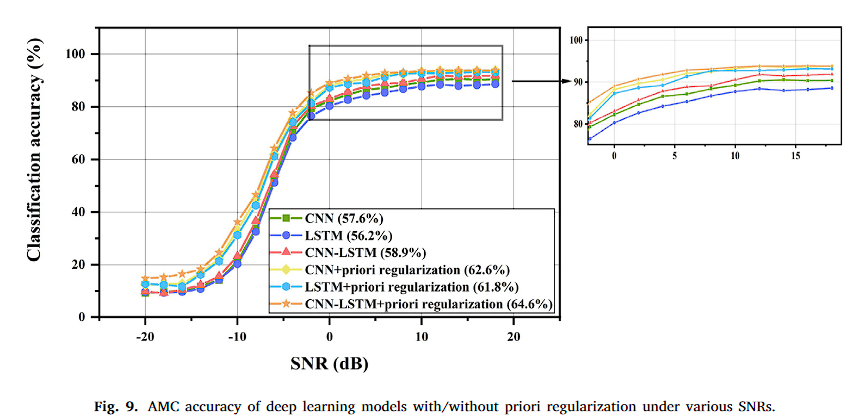
本文的实验结果和论文1的结果比较类似,即使without priori regularization
2、论文2

五、总结
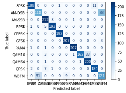
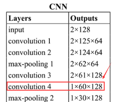
- 对于RadioML2016.10a数据集来说,在信噪比不是特别低的情况下,使用CNN就表现的不错,在SNR=6dB可达91.82%,但是这里有个小技巧,在卷积过程中,先单独对IQ分量进行卷积,在convolution 4进行联合处理,一开始就使用2x2的卷积核效果较差。
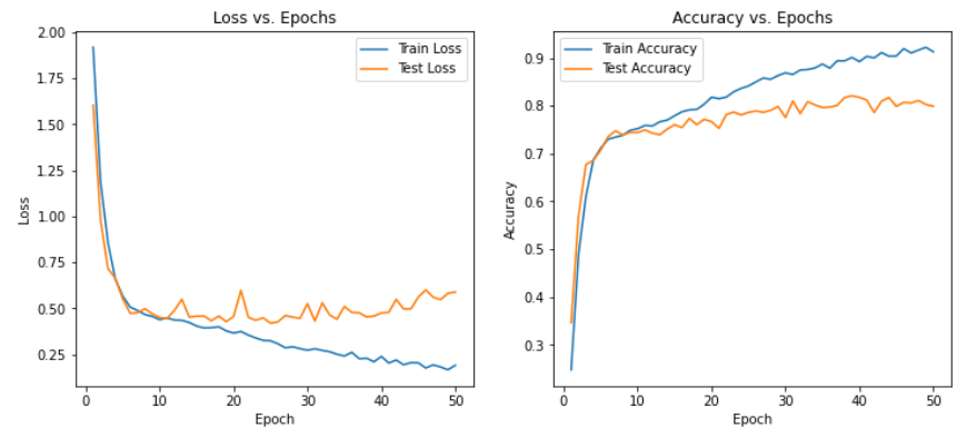
- 实验结果表明,CNN+LSTM 优于 CNN,但涨幅不多
- 完整的代码和数据集在GIthub:https://github.com/daetz-coder/RadioML2016.10a_Benchmark,为了方便使用,IQ分量保存在csv中,且仅提供了SNR=6dB的数据,如果需要更多类型的数据,请参考https://blog.csdn.net/a_student_2020/article/details/139800725