文章目录
- 🚗 II. Overview of the decision-making hierarchy used in driverless cars(无人驾驶汽车的决策层综述)
- 🔴 A. Route Planning(路径规划)
- 🟠 B. Behavioral Decision Making(行为决策)
- 🟡 C. Motion Planning(运动规划)
- 🟢 D. Vehicle Control(车辆控制)
- 🚚 III. Modeling for planning and control (规划与控制的建模)
- 🔴 A. The Kinematic Single-Track Model(单轨运动学模型)
- 🟠 B. Inertial Effects(惯性效应)
🚗 II. Overview of the decision-making hierarchy used in driverless cars(无人驾驶汽车的决策层综述)
In this section we describe the decision making architecture of a typical self-driving car and comment on the responsibilities of each component. Driverless cars are essentially autonomous decision-making systems that process a stream of observations from on-board sensors such as radars, LIDARs, cameras, GPS/INS units, and odometry. These observations, together with prior knowledge about the road network, rules of the road, vehicle dynamics, and sensor models, are used to automatically select values for controlled variables governing the vehicle’s motion. Intelligent vehicle research aims at automating as much of the driving task as possible. The commonly adopted approach to this problem is to partition and organize perception and decision-making tasks into a hierarchical structure. The prior information and collected observation data are used by the perception system to provide an estimate of the state of the vehicle and its surrounding environment; the estimates are then used by the decision-making system to control the vehicle so that the driving objectives are accomplished.
在本节中,我们将描述典型的自动驾驶汽车的决策层架构,并讨论其中每个组成部分的作用。无人驾驶汽车本质上是一种自主决策系统,它处理来自雷达、激光雷达(LIDARs)、相机、GPS/INS(全球定位系统/惯性导航系统)单元和里程计等车载传感器的观测流。这些观测结果与关于道路网络、道路规则、车辆动力学和传感器模型的先验知识一起,用于自动选择控制车辆运动的受控变量的取值。智能汽车研究旨在尽可能多地实现驾驶任务的自动化。解决这个问题的常用方法是将感知和决策任务划分并组织成一个层次结构。感知系统使用先验信息和收集的观测数据,来提供车辆及其周围环境的状态估计。决策系统随后使用这些估计来控制车辆,从而实现驾驶目标。
The decision making system of a typical self-driving car is hierarchically decomposed into four components (cf. Figure II.1): At the highest level a route is planned through the road network. This is followed by a behavioral layer, which decides on a local driving task that progresses the car towards the destination and abides by rules of the road. A motion planning module then selects a continuous path through the environment to accomplish a local navigational task. A control system then reactively corrects errors in the execution of the
planned motion. In the remainder of the section we discuss the responsibilities of each of these components in more detail.
典型的自动驾驶汽车的决策系统依据层级分解为四个组成部分(参考图II.1):在最高层,系统通过道路网络规划出一条路线;随后的行为层指定一个局部驾驶任务,使汽车朝着目的地前进同时遵守道路规则;随后,运动规划模块选择一条通过环境的连续路径,以完成局部导航任务;最后,控制系统反应性地修正执行规划运动时的误差。本节的其余部分将更详细地讨论每个组成部分的作用。

图II.1:决策过程的层级。根据目的地,路线规划器通过道路网络生成一条路线。行为层对环境进行推理,并生成沿着所选路线前进的运动规范。运动规划器随后求解实现规范的可行运动。反馈控制对致动变量进行调参,以修正执行参考路径时的误差。
🔴 A. Route Planning(路径规划)
At the highest level, a vehicle’s decision-making system must select a route through the road network from its current position to the requested destination. By representing the road network as a directed graph with edge weights corresponding to the cost of traversing a road segment, such a route can be formulated as the problem of finding a minimum-cost path on a road network graph. The graphs representing road networks can however contain millions of edges making classical shortest path algorithms such as Dijkstra [32] or A* [33] impractical. The problem of efficient route planning in transportation networks has attracted significant interest in the transportation science community leading to the invention of a family of algorithms that after a one-time pre-processing step return an optimal route on a continent-scale network in milliseconds [34], [35]. For a comprehensive survey and comparison of practical algorithms that can be used to efficiently plan routes for both human-driven and self-driving vehicles, see [36].
在最高层上,车辆的决策系统必须选择一条从当前位置到请求的目的地的、通过道路网络的路线。通过将道路网络表示为一个有向图(有向图的边的权重对应所穿过的道路段的成本),可以将路线规划问题构造为在道路网络图上找到一条最小成本路径的问题。然而,表示道路网络的图可以包含数百万条边,使得经典的最短路径算法(如Dijkstra [32]或A * [33])不再实用。交通网络中的高效路线规划问题引起了交通科学界的极大兴趣,催生了一系列算法。这些算法经过一次性的预处理步骤后,能够在毫秒时间内返回大陆规模的道路网络上的一条最优路线[34][35]。有关可用于高效的人类驾驶和自动驾驶车辆路线规划的实用算法的全面综述和比较,请参考[36]。
🟠 B. Behavioral Decision Making(行为决策)
After a route plan has been found, the autonomous vehicle must be able to navigate the selected route and interact with other traffic participants according to driving conventions and rules of the road. Given a sequence of road segments specifying the selected route, the behavioral layer is responsible for selecting an appropriate driving behavior at any point of time based on the perceived behavior of other traffic participants, road conditions, and signals from infrastructure. For example, when the vehicle is reaching the stop line before an intersection, the behavioral layer will command the vehicle to come to a stop, observe the behavior of other vehicles, bikes, and pedestrians at the intersection, and let the vehicle proceed once it is its turn to go.
找到一条路线计划后,自动驾驶车辆必须能够根据驾驶惯例和道路规则来导航选定的路线并与其他交通参与者进行交互。当给定了指定所选路线的一系列路段时,行为层基于感知到的其他交通参与者的行为、道路状况和基础设施信号,负责在任何时间点选择适当的驾驶行为。例如,当车辆在交叉路口前到达停车线时,行为层将命令车辆停车,观察交叉路口的其他车辆、自行车和行人的行为,并在轮到车辆行驶时让车辆继续前进。
Driving manuals dictate qualitative actions for specific driving contexts. Since both driving contexts and the behaviors available in each context can be modeled as finite sets, a natural approach to automating this decision making is to model each behavior as a state in a finite state machine with transitions governed by the perceived driving context such as relative position with respect to the planned route and nearby vehicles. In fact, finite state machines coupled with different heuristics specific to considered driving scenarios were adopted as a mechanism for behavior control by most teams in the DARPA Urban Challenge [9].
驾驶手册规定了特定驾驶环境下的定性行动。由于驾驶环境和每个环境中可用的行为都可以被建模为有限集,因此自动化这种决策的一种自然方法是将每个行为建模为有限状态机中的状态,其中状态的转移受感知到的驾驶环境的控制,这些驾驶环境包括相对于规划的路线和附近车辆的相对位置。事实上,在DARPA城市挑战赛中,大多数团队采用了有限状态机和特定于所考虑驾驶场景的不同启发式,作为行为控制的机制[9]。
Real-world driving, especially in an urban setting, is however characterized by uncertainty over the intentions of other traffic participants. The problem of intention prediction and estimation of future trajectories of other vehicles, bikes and pedestrians has also been studied. Among the proposed solution techniques are machine learning based techniques, e.g., Gaussian mixture models [37], Gaussian process regression [38] and the learning techniques reportedly used in Google’s self-driving system for intention prediction [39], as well as model-based approaches for directly estimating intentions from sensor measurements [40], [41].
然而,现实世界(尤其是城市环境)的驾驶的特点是,其他交通参与者的意图(intentions)具有不确定性。因此,学界还研究了对其他车辆、自行车和行人的未来轨迹的意图预测和估计。提出的解决方案包括基于机器学习的技术,例如高斯混合模型[37]、高斯过程回归[38]、被报道的在谷歌自动驾驶系统中用于意图预测的学习技术[39],以及用于从传感器测量值中直接估计意图的基于模型的方法[40][41]。
This uncertainty in the behavior of other traffic participants is commonly considered in the behavioral layer for decision making using probabilistic planning formalisms, such as Markov Decision Processes (MDPs) and generalizations. For example, [42] formulates the behavioral decision-making problem in MDP framework. Several works [43]–[46] model unobserved different driving scenarios and pedestrian intentions explicitly using a partially-observable Markov decision process (POMDP) framework and propose specific approximate solution strategies.
其他交通参与者行为的这种不确定性通常在使用概率规划形式(如马尔可夫决策过程(MDPs)及其推广形式)进行决策的行为层中被考虑。例如,文章[42]在MDP框架中构造了行为决策问题。一些工作[43–46]使用部分可观察马尔可夫决策过程(POMDP)框架,以显式地模拟未观察到的驾驶场景和行人意图,并提出了具体的近似解决策略。
🟡 C. Motion Planning(运动规划)
When the behavioral layer decides on the driving behavior to be performed in the current context, which could be, e.g., cruise-in-lane, change-lane, or turn-right, the selected behavior has to be translated into a path or trajectory that can be tracked by the low-level feedback controller. The resulting path or trajectory must be dynamically feasible for the vehicle, comfortable for the passenger, and avoid collisions with obstacles detected by the on-board sensors. The task of finding such a path or trajectory is a responsibility of the motion planning system, which is discussed in greater detail in Section IV.
行为层决定的要在当前环境中执行的驾驶行为(例如车道巡航、变道或右转)必须被转换为一条可由低级反馈控制器跟踪的路径或轨迹。生成的路径或轨迹对于车辆必须是动态可行的,同时可以保证乘客的舒适,并避免与车载传感器检测到的障碍物发生碰撞。找到这样的一条路径或轨迹是运动规划系统的工作,这将在第四节中详细讨论。
🟢 D. Vehicle Control(车辆控制)
In order to execute the reference path or trajectory from the motion planning system a feedback controller is used to select appropriate actuator inputs to carry out the planned motion and correct tracking errors. The tracking errors generated during the execution of a planned motion are due in part to the inaccuracies of the vehicle model. Thus, a great deal of emphasis is placed on the robustness and stability of the closed loop system.
为了执行来自运动规划系统的参考路径或轨迹,使用反馈控制器来选择适当的致动器输入。执行规划运动期间会产生跟踪误差的部分原因是车辆模型不够准确。因此,闭环系统的鲁棒性和稳定性受到了极高的重视。
Many effective feedback controllers have been proposed for executing the reference motions provided by the motion planning system. A survey of related techniques are discussed in detail in Section V.
目前已经提出了许多有效的反馈控制器,用于执行由运动规划系统提供的参考运动。第5节详细讨论了相关技术的概况。
🚚 III. Modeling for planning and control (规划与控制的建模)
In this section we will survey the most commonly used models of mobility of car-like vehicles. Such models are widely used in control and motion planning algorithms to approximate a vehicle’s behavior in response to control actions in relevant operating conditions. A high-fidelity model may accurately reflect the response of the vehicle, but the added detail may complicate the planning and control problems.This presents a trade-off between the accuracy of the selected model and the difficulty of the decision problems. This section provides an overview of general modeling concepts and a survey of models used for motion planning and control.
在本节中,我们将综述最常用的类车车辆(car-like vehicles)的移动模型。此类模型被广泛用于控制和运动规划算法,来近似在相关操作条件下响应于控制动作的车辆行为。高保真模型可以准确地反映车辆的响应,但增加的细节可能会使规划和控制问题复杂化。这要求在所选模型的准确性和决策问题的难度之间做出权衡。本节将对通用的建模概念进行概述,同时将综述用于运动规划和控制的模型。
Modeling begins with the notion of the vehicle configuration, representing its pose or position in the world. For example, configuration can be expressed as the planar coordinate of a point on the car together with the car’s heading. This is a coordinate system for the onfiguration space of the car. This coordinate system describes planar rigid-body motions (represented by the Special Euclidean group in two dimensions, SE(2)) and is a commonly used configuration space [47]–[49]. Vehicle motion must then be planned and regulated to accomplish driving tasks and while respecting the constraints introduced by the selected model.
建模的第一步是车辆构型/配置(configuration)的概念,它表示车辆在世界中的位姿或位置。例如可以用汽车上某一点的平面坐标以及汽车的方向来表示其构型,这便是汽车的构型空间/配置空间(configuration space / C-space)的坐标系。该坐标系描述平面刚体运动(表示为二维的特殊欧氏群 SE(2) ),是常用的构型空间[47-49]。随后,对车辆运动进行规划和控制,以完成驾驶任务,同时必须满足所选模型引入的约束。
🔴 A. The Kinematic Single-Track Model(单轨运动学模型)
In the most basic model of practical use, the car consists of two wheels connected by a rigid link and is restricted to move in a plane [48]–[52]. It is assumed that the wheels do not slip at their contact point with the ground, but can rotate freely about their axes of rotation. The front wheel has an added degree of freedom where it is allowed to rotate about an axis normal to the plane of motion. This is to model steering. These two modeling features reflect the experience most passengers have where the car is unable to make lateral displacement without simultaneously moving forward. More formally, the limitation on maneuverability is referred to as a nonholonomic constraint [47], [53]. The nonholonomic constraint is expressed as a differential constraint on the motion of the car. This expression varies depending on the choice of coordinate system. Variations of this model have been referred to as the car-like robot, bicycle model, kinematic model, or single track model.
实践使用的最基础的汽车模型由两个通过刚性连杆连接的车轮组成,并且被限制在平面内移动[48-52]。该模型假设车轮在其与地面的接触点处不会滑动,但可以绕其旋转轴自由旋转。前轮具有额外的自由度,允许其绕垂直于运动平面的轴旋转,以模拟转向。这两个建模特征反映了大多数乘客的体验,即汽车无法在不向前移动的同时实现横向位移。更正式地,这种机动性限制被称为非完整约束[47][53]。非完整约束表示为汽车运动的微分约束,约束的表达式随坐标系的选择而变化。这种汽车模型的变体被称为类车机器人、自行车模型、运动学模型或单轨模型。
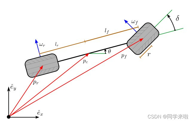
The following is a derivation of the differential constraint in several popular coordinate systems for the configuration. In reference to Figure III.1, the vectors
p
r
p_r
pr and
p
f
p_f
pf denote the location of the rear and front wheels in a stationary or inertial coordinate system with basis vectors
(
e
^
x
,
e
^
y
,
e
^
z
)
\left(\hat{e}_x, \hat{e}_y, \hat{e}_z\right)
(e^x,e^y,e^z). The heading
θ
\theta
θ is an angle describing the direction that the vehicle is facing. This is defined as the angle between vectors
e
^
x
\hat{e}_x
e^x and
p
f
−
p
r
p_f-p_r
pf−pr.
接下来我们将推导这种构型在几种常用坐标系中的微分约束。参考图III.1,向量
p
r
p_r
pr 和
p
f
p_f
pf 分别表示静止坐标系或惯性坐标系中后轮和前轮的位置,坐标系由三个基向量
(
e
^
x
,
e
^
y
,
e
^
z
)
\left(\hat{e}_x, \hat{e}_y, \hat{e}_z\right)
(e^x,e^y,e^z) 所决定。航向
θ
\theta
θ 是描述车辆朝向的角度,定义为向量
e
^
x
\hat{e}_x
e^x 和
p
f
−
p
r
p_f-p_r
pf−pr 的夹角。
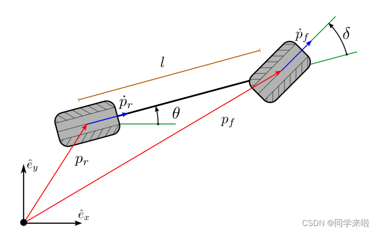
图III.1:单轨模型的运动学,其中 p r p_r pr 和 p f p_f pf分别是后轮和前轮与地面的接触点, θ \theta θ 是车辆航向, δ \delta δ 是前轮的转向角。由于非完整约束, p r p_r pr 和 p f p_f pf 的时间导数被限制在蓝色箭头指示的方向上。
Differential constraints will be derived for the coordinate systems consisting of the angle
θ
\theta
θ, together with the motion of one of the points
p
r
p_r
pr as in [54], and
p
f
p_f
pf as in [55].
一个坐标系下的微分约束的表达式包括该坐标系下的角度
θ
\theta
θ 以及车辆上一点的运动,如向量
p
r
p_r
pr(参考[54])或
p
f
p_f
pf(参考[55])。
The motion of the points
p
r
p_r
pr and
p
f
p_f
pf must be collinear with the wheel orientation to satisfy the no-slip assumption. Expressed as an equation, this constraint on the rear wheel is
点
p
r
p_r
pr 和
p
f
p_f
pf 的运动必须与车轮的朝向共线,以满足无滑移假设。对于后轮的该约束可以表示为
(
p
˙
r
⋅
e
^
y
)
cos
(
θ
)
−
(
p
˙
r
⋅
e
^
x
)
sin
(
θ
)
=
0
(
I
I
I
.
1
)
\left(\dot{p}_r \cdot \hat{e}_y\right) \cos (\theta)-\left(\dot{p}_r \cdot \hat{e}_x\right) \sin (\theta)=0 \quad(III.1)
(p˙r⋅e^y)cos(θ)−(p˙r⋅e^x)sin(θ)=0(III.1)
and for the front wheel:
对于前轮的该约束可以表示为
(
p
˙
f
⋅
e
^
y
)
cos
(
θ
+
δ
)
−
(
p
˙
f
⋅
e
^
x
)
sin
(
θ
+
δ
)
=
0
(
I
I
I
.
2
)
\left(\dot{p}_f \cdot \hat{e}_y\right) \cos (\theta+\delta)-\left(\dot{p}_f \cdot \hat{e}_x\right) \sin (\theta+\delta)=0 \quad(III.2)
(p˙f⋅e^y)cos(θ+δ)−(p˙f⋅e^x)sin(θ+δ)=0(III.2)
This expression is usually rewritten in terms of the component-wise motion of each point along the basis vectors. The motion of the rear wheel along the
e
^
x
\hat{e}_x
e^x-direction is
x
r
:
=
p
r
⋅
e
^
x
x_r:=p_r \cdot \hat{e}_x
xr:=pr⋅e^x. Similarly, for
e
^
y
\hat{e}_y
e^y-direction,
y
r
:
=
p
r
⋅
e
^
y
y_r:=p_r \cdot \hat{e}_y
yr:=pr⋅e^y. The forward speed is
v
r
:
=
p
˙
r
⋅
(
p
f
−
p
r
)
/
∥
(
p
f
−
p
r
)
∥
v_r:=\dot{p}_r \cdot\left(p_f-p_r\right) /\left\|\left(p_f-p_r\right)\right\|
vr:=p˙r⋅(pf−pr)/∥(pf−pr)∥, which is the magnitude of
p
˙
r
\dot{p}_r
p˙r with the correct sign to indicate forward or reverse driving. In terms of the scalar quantities
x
r
x_r
xr ,
y
r
y_r
yr , and
θ
\theta
θ, the differential constraint is
利用每个点沿基向量的运动分量,可以重写上式。后轮沿
e
^
x
\hat{e}_x
e^x方向的运动可以写作
x
r
:
=
p
r
⋅
e
^
x
x_r:=p_r \cdot \hat{e}_x
xr:=pr⋅e^x,相似地,沿
e
^
y
\hat{e}_y
e^y 方向的运动写作
y
r
:
=
p
r
⋅
e
^
y
y_r:=p_r \cdot \hat{e}_y
yr:=pr⋅e^y 。前向速度
v
r
:
=
p
˙
r
⋅
(
p
f
−
p
r
)
/
∥
(
p
f
−
p
r
)
∥
v_r:=\dot{p}_r \cdot\left(p_f-p_r\right) /\left\|\left(p_f-p_r\right)\right\|
vr:=p˙r⋅(pf−pr)/∥(pf−pr)∥,表示
p
˙
r
\dot{p}_r
p˙r的大小,同时带有正确的正负号,该正负号用于描述当前的行驶是正向或反向驾驶。利用
x
r
x_r
xr ,
y
r
y_r
yr 和
θ
\theta
θ这几个标量,微分约束可以写作
x
˙
r
=
v
r
cos
(
θ
)
y
˙
r
=
v
r
sin
(
θ
)
θ
˙
=
v
r
l
tan
(
δ
)
(
I
I
I
.
3
)
\begin{aligned} \\ & \dot{x}_r=v_r \cos (\theta) \\ & \dot{y}_r=v_r \sin (\theta) \\ & \dot{\theta}=\frac{v_r}{l} \tan (\delta)\end{aligned} \quad(III.3)
x˙r=vrcos(θ)y˙r=vrsin(θ)θ˙=lvrtan(δ)(III.3)
Alternatively, the differential constraint can be written in terms the motion of
p
f
p_f
pf,
类似地,也可以利用
p
f
p_f
pf的运动将微分约束写作
x
˙
f
=
v
f
cos
(
θ
+
δ
)
y
˙
f
=
v
f
sin
(
θ
+
δ
)
θ
˙
=
v
f
l
sin
δ
(
I
I
I
.
4
)
\begin{aligned} &\dot{x}_f=v_f \cos (\theta+\delta) \\ &\dot{y}_f=v_f \sin (\theta+\delta) \\ &\dot{\theta}=\frac{v_f}{l} \sin \delta \end{aligned} \quad(III.4)
x˙f=vfcos(θ+δ)y˙f=vfsin(θ+δ)θ˙=lvfsinδ(III.4)
where the front wheel forward speed
v
f
v_f
vf is now used. The front wheel speed,
v
r
v_r
vr , is related to the rear wheel speed by
其中
v
f
v_f
vf是前轮的前向速度,它与后轮速度
v
r
v_r
vr满足关系
v
r
v
f
=
cos
(
δ
)
(
I
I
I
.
5
)
\frac{v_r}{v_f}=\cos (\delta) \quad(III.5)
vfvr=cos(δ)(III.5)
The planning and control problems for this model involve selecting the steering angle
δ
\delta
δ within the mechanical limits of the vehicle
δ
∈
[
δ
min
,
δ
max
]
\delta \in\left[\delta_{\min }, \delta_{\max }\right]
δ∈[δmin,δmax], and forward speed
v
r
v_r
vr within an acceptable range,
v
r
∈
[
v
min
,
v
max
]
v_r \in\left[v_{\min }, v_{\max }\right]
vr∈[vmin,vmax].
利用这个模型求解规划和控制问题涉及在车辆的机械限制范围内选择转向角
δ
∈
[
δ
min
,
δ
max
]
\delta \in\left[\delta_{\min }, \delta_{\max }\right]
δ∈[δmin,δmax],以及在合适的范围内选择前向速度
v
r
∈
[
v
min
,
v
max
]
v_r \in\left[v_{\min }, v_{\max }\right]
vr∈[vmin,vmax]。
A simplification that is sometimes utilized, e.g. [56], is to select the heading rate
ω
\omega
ω instead of steering angle
δ
\delta
δ. These quantities are related by
一种经常采用的简化方式是选择一个航向率
ω
\omega
ω 而非选择一个转向角
δ
\delta
δ 。这些变量满足关系
δ
=
arctan
l
ω
v
r
(
I
I
I
.
6
)
\delta=\arctan \frac{l \omega}{v_r} \quad(III.6)
δ=arctanvrlω(III.6)
simplifying the heading dynamics to
并随之得以将转向动力学简化为
θ
˙
=
ω
,
ω
∈
[
v
r
l
tan
δ
min
,
v
r
l
tan
δ
max
]
(
I
I
I
.
7
)
\dot{\theta}=\omega, \quad \omega \in\left[\frac{v_r}{l} \tan \delta_{\min }, \frac{v_r}{l} \tan \delta_{\max }\right] \quad(III.7)
θ˙=ω,ω∈[lvrtanδmin,lvrtanδmax](III.7)
In this situation, the model is sometimes referred to as the unicycle model since it can be derived by considering the motion of a single wheel.
此时的模型经常被称为单轮(unicycle)模型,因为它的推导相当于只考虑了一个轮子的运动。
An important variation of this model is the case when
v
r
v_r
vr is fixed. This is sometimes referred to as the Dubins car, after Lester Dubins who derived the minimum time motion between to points with prescribed tangents [57]. Another notable variation is the Reeds-Shepp car for which minimum length paths are known when
v
r
v_r
vr takes a single forward and reverse speed [58]. These two models have proven to be of some importance to motion planning and will be discussed further in Section IV.
该模型的一个重要变体是
v
r
v_r
vr 固定时的情况,此时的模型又被称为Dubins车(Dubins Car),以纪念Lester Dubins推导出了具有指定切线的两点之间的最小时间运动[57]。另一个值得注意的变体是Reeds-Shepp车,此时对于最短路径的求解允许
v
r
v_r
vr 是正向或者反向行驶的速度[58]。这两种模型已被证明对运动规划具有一定的重要性,因此将在第四节中作进一步讨论。
The kinematic models are suitable for planning paths at low speeds (e.g. parking maneuvers and urban driving) where inertial effects are small in comparison to the limitations on mobility imposed by the no-slip assumption. A major drawback of this model is that it permits instantaneous steering angle changes which can be problematic if the motion planning module generates solutions with such instantaneous changes.
运动学模型适用于低速(例如泊车和城市驾驶)下的路径规划。在这些低速行驶的场景中,相比于无滑移假设对移动性的限制,惯性效应较小。该模型的主要缺点是它允许瞬时的转向角变化:如果运动规划模块生成具有这种瞬时变化的解,可能将带来很多麻烦。
Continuity of the steering angle can be imposed by augmenting (III.4), where the steering angle integrates a commanded rate as in [49]. Equation (III.4) becomes
转向角的连续性可以通过增强方程(3.4)来实现,其中转向角被处理为指定速率的积分,参考[49]。方程(3.4)进而变为
x
˙
f
=
v
f
cos
(
θ
+
δ
)
y
˙
f
=
v
f
sin
(
θ
+
δ
)
θ
˙
=
v
f
l
sin
δ
δ
˙
=
v
δ
(
I
I
I
.
8
)
\begin{aligned} &\dot{x}_f=v_f \cos (\theta+\delta) \\ &\dot{y}_f=v_f \sin (\theta+\delta) \\ &\dot{\theta}=\frac{v_f}{l} \sin \delta \\ & \dot{\delta}=v_\delta \end{aligned}\quad(III.8)
x˙f=vfcos(θ+δ)y˙f=vfsin(θ+δ)θ˙=lvfsinδδ˙=vδ(III.8)
In addition to the limit on the steering angle, the steering rate can now be limited:
v
δ
∈
[
δ
˙
min
,
δ
˙
max
]
v_\delta \in\left[\dot{\delta}_{\min }, \dot{\delta}_{\max }\right]
vδ∈[δ˙min,δ˙max]. The same problem can arise with the car’s speed
v
r
v_r
vr and can be resolved in the same way. The drawback to this technique is the increased dimension of the model which can complicate motion planning and control problems.
此时除了限制转向角,还要约束转向率
v
δ
∈
[
δ
˙
min
,
δ
˙
max
]
v_\delta \in\left[\dot{\delta}_{\min }, \dot{\delta}_{\max }\right]
vδ∈[δ˙min,δ˙max]。同样的问题也可能发生在车速
v
r
v_r
vr上,但可以通过与转向角相同的方式来解决。这种方法的缺点是增加了模型的维度,使得运动规划与控制问题被复杂化了。
While the kinematic bicycle model and simple variations are very useful for motion planning and control, models considering wheel slip [59], inertia [18], [60]–[62], and chassis dynamics [60] can better utilize the vehicle’s capabilities for executing agile maneuvers. These effects become significant when planning motions with high acceleration and jerk.
坐标系的选择并不限定必须选择一个轮子的位置作为车辆的位置坐标。对于通过经典力学原理推导得到的模型,使用质心作为位置坐标可能更加方便,参考[59][60],或者使用摆心,参考[61][62]。
🟠 B. Inertial Effects(惯性效应)
When the acceleration of the vehicle is sufficiently large, the no-slip assumption between the tire and ground becomes invalid. In this case a more accurate model for the vehicle is as a rigid body satisfying basic momentum principles. That is, the acceleration is proportional to the force generated by the ground on the tires. Taking
p
c
p_c
pc to be the vehicles center of mass, and a coordinate of the configuration (cf. Figure III.2), the motion of the vehicle is governed by
当车辆的加速度足够大时,轮胎与地面之间的无滑移假设不再成立。此时,一个更加准确的模型是将车辆视为一个满足动量定理的刚体,即,加速度正比于地面施加在轮胎上的力。取
p
c
p_c
pc 作为车辆的质心以及构型坐标(参考图3.2),车辆的运动有以下关系:
m
p
¨
c
=
F
f
+
F
r
I
z
z
θ
¨
=
(
p
c
−
p
f
)
×
F
f
+
(
p
c
−
p
r
)
×
F
r
(
I
I
I
.
9
)
\begin{aligned} &m \ddot{p}_c=F_f+F_r \\ & I_{z z} \ddot{\theta}=\left(p_c-p_f\right) \times F_f+\left(p_c-p_r\right) \times F_r \end{aligned}\quad(III.9)
mp¨c=Ff+FrIzzθ¨=(pc−pf)×Ff+(pc−pr)×Fr(III.9)
where
F
r
F_r
Fr and
F
f
F_f
Ff are the forces applied to the vehicle by the ground through the ground-tire interaction,
m
m
m is the vehicles total mass, and
I
z
z
I_{zz}
Izz is the polar moment of inertia in the
e
^
z
\hat{e}_z
e^z direction about the center of mass. In the following derivations we tacitly neglect the motion of
p
c
p_c
pc in the
e
^
z
\hat{e}_z
e^z direction with the assumptions that the road is level, the suspension is rigid and vehicle remains on the road.
其中
F
r
F_r
Fr和
F
f
F_f
Ff是地面通过与轮胎的接触而施加于车辆的力,
m
m
m是车辆的总质量,
I
z
z
I_{zz}
Izz是在
e
^
z
\hat{e}_z
e^z方向上关于质心的极惯性矩。在接下来的推导中,我们将基于平坦地面、刚体悬架以及车辆保持在道路上的假设,默认忽略
p
c
p_c
pc在
e
^
z
\hat{e}_z
e^z方向上的运动。
The expressions for Fr and Ff vary depending on modeling assumptions [18], [59], [60], [62], but in any case the expression can be tedious to derive. Equations (III.10)-(III.15) therefore provide a detailed derivation as a reference.
F
r
F_r
Fr和
F
f
F_f
Ff的表达式随建模假设[18][59][60][62]而变化,但在任何情况下,推导该表达式都可能很繁琐。因此,方程(III.10)-(III.15)提供了详细的推导作为参考。
The force between the ground and tires is modeled as being dependent on the rate that the tire slips on the ground. Although the center of mass serves as a coordinate for the configuration, the velocity of each wheel relative to the ground is needed to determine this relative speed. The kinematic relations between these three points are
地面与轮胎之间的力被建模为与轮胎在地面上滑动的速率有关。尽管选择质心作为构型的坐标,但仍然需要每个车轮相对于地面的速度,以确定该相对速度。这三个点之间的运动学关系为
p
r
=
p
c
+
(
−
l
r
cos
θ
−
l
r
sin
θ
0
)
p
˙
r
=
p
˙
c
+
(
0
0
θ
˙
)
×
(
−
l
r
cos
θ
−
l
r
sin
θ
0
)
p
f
=
p
c
+
(
l
f
cos
θ
l
f
sin
θ
0
)
p
˙
f
=
p
˙
c
+
(
0
0
θ
˙
)
×
(
l
f
cos
θ
l
f
sin
θ
0
)
(
I
I
I
.
10
)
\begin{aligned} &p_r=p_c+\left(\begin{array}{c} -l_r \cos \theta \\ -l_r \sin \theta \\ 0 \end{array}\right) \\ & \dot{p}_r=\dot{p}_c+\left(\begin{array}{c} 0 \\ 0 \\ & \dot{\theta} \end{array}\right) \times\left(\begin{array}{c} -l_r \cos \theta \\ -l_r \sin \theta \\ 0 \end{array}\right) \\ &p_f=p_c+\left(\begin{array}{c} l_f \cos \theta \\ l_f \sin \theta \\ 0 \end{array}\right) \\ &\dot{p}_f=\dot{p}_c+\left(\begin{array}{c} 0 \\ 0 \\ \dot{\theta} \end{array}\right) \times\left(\begin{array}{c} l_f \cos \theta \\ l_f \sin \theta \\ 0 \end{array}\right) \end{aligned}\quad(III.10)
pr=pc+
−lrcosθ−lrsinθ0
p˙r=p˙c+
00θ˙
×
−lrcosθ−lrsinθ0
pf=pc+
lfcosθlfsinθ0
p˙f=p˙c+
00θ˙
×
lfcosθlfsinθ0
(III.10)
These kinematic relations are used to determine the velocities of the point on each tire in contact with the ground,
s
r
s_r
sr and
s
f
s_f
sf . The velocity of these points are referred to as the tire slip velocity. In general,
s
r
s_r
sr and
s
f
s_f
sf differ from
p
˙
r
\dot{p}_r
p˙r and
p
˙
f
\dot{p}_f
p˙f through the angular velocity of the wheel. The kinematic relation is
这些运动学关系用于确定每个轮胎与地面的接触点的速度
s
r
s_r
sr 和
s
f
s_f
sf 。这些点的速度又被称为轮胎滑动速度。通常,由于存在轮胎的角速度,因此
s
r
s_r
sr 和
s
f
s_f
sf 不同于
p
˙
r
\dot{p}_r
p˙r 和
p
˙
f
\dot{p}_f
p˙f 。它们之间的运动学关系如下:
s
r
=
p
˙
r
+
ω
r
×
R
s
f
=
p
˙
f
+
ω
f
×
R
(
I
I
I
.
11
)
\begin{aligned} & s_r=\dot{p}_r+\omega_r \times R \\ & s_f=\dot{p}_f+\omega_f \times R \end{aligned}\quad(III.11)
sr=p˙r+ωr×Rsf=p˙f+ωf×R(III.11)
The angular velocities of the wheels are given by
其中车轮的角速度由下式给出:
ω
r
=
(
Ω
r
sin
θ
−
Ω
r
cos
θ
0
)
,
ω
f
=
(
Ω
f
sin
(
θ
+
δ
)
−
Ω
f
cos
(
θ
+
δ
)
0
)
(
I
I
I
.
12
)
\omega_r=\left(\begin{array}{c} \Omega_r \sin \theta \\ -\Omega_r \cos \theta \\ 0 \end{array}\right), \quad \omega_f=\left(\begin{array}{c} \Omega_f \sin (\theta+\delta) \\ -\Omega_f \cos (\theta+\delta) \\ 0 \end{array}\right) \quad(III.12)
ωr=
Ωrsinθ−Ωrcosθ0
,ωf=
Ωfsin(θ+δ)−Ωfcos(θ+δ)0
(III.12)
and
R
=
(
0
,
0
,
−
r
)
T
R=(0,0,-r)^T
R=(0,0,−r)T . The wheel radius is the scalar quantity
r
r
r, and
Ω
{
r
,
f
}
\Omega_{\{r, f\}}
Ω{r,f} are the angular speeds of each wheel relative to the car. This is illustrated for the rear wheel in Figure III.3
且
R
=
(
0
,
0
,
−
r
)
T
R=(0,0,-r)^T
R=(0,0,−r)T 。车轮半径用标量
r
r
r 表示,每个轮胎相对于汽车的角速率用
Ω
{
r
,
f
}
\Omega_{\{r, f\}}
Ω{r,f} 表示。图3.3描绘了后轮上的各个变量之间的关系。
图III.2:没有无滑移假设的单轨模型的运动学图解,其中 ω { r , f } \omega_{\{r, f\}} ω{r,f} 是车轮相对于车辆的相对角速度

图III.3:二维的后轮运动学图解表明了车轮滑移 S r S_r Sr 与后轮速度 p ˙ r \dot{p}_r p˙r 以及角速率
Under static conditions, or when the height of the center of mass can be approximated as
p
c
⋅
e
^
z
≈
0
p_c \cdot \hat{e}_z \approx 0
pc⋅e^z≈0, the component of the force normal to the ground,
F
{
r
,
f
}
⋅
e
^
z
F_{\{r, f\}} \cdot \hat{e}_z
F{r,f}⋅e^z can be computed from a static force-torque balance as
在静态条件下,或者当质心的高度可以近似满足
p
c
⋅
e
^
z
≈
0
p_c \cdot \hat{e}_z \approx 0
pc⋅e^z≈0 时,地面施加给轮胎的力在垂直于地面的方向上的分量
F
{
r
,
f
}
⋅
e
^
z
F_{\{r, f\}} \cdot \hat{e}_z
F{r,f}⋅e^z 可以通过静力学的力矩平衡而给出:
F
f
⋅
e
^
z
=
l
r
m
g
l
f
+
l
r
,
F
r
⋅
e
^
z
=
l
f
m
g
l
f
+
l
r
(
I
I
I
.
13
)
F_f \cdot \hat{e}_z=\frac{l_r m g}{l_f+l_r}, \quad F_r \cdot \hat{e}_z=\frac{l_f m g}{l_f+l_r} \quad(III.13)
Ff⋅e^z=lf+lrlrmg,Fr⋅e^z=lf+lrlfmg(III.13)
The normal force is then used to compute the traction force on each tire together with the slip and a friction coefficient model,
μ
\mu
μ, for the tire behavior. The traction force on the rear tire is given component-wise by
法向力随后同滑移以及一个描述轮胎特性的摩擦系数模型
μ
\mu
μ 一起,用于计算每个轮胎上的牵引力。后轮上的牵引力的分量给出如下:
F
r
⋅
e
^
x
=
−
(
F
r
⋅
e
^
z
)
μ
(
∥
s
r
∥
Ω
r
r
)
s
r
∥
s
r
∥
⋅
e
^
x
F
r
⋅
e
^
y
=
−
(
F
r
⋅
e
^
z
)
μ
(
∥
s
r
∥
Ω
r
r
)
s
r
∥
s
r
∥
⋅
e
^
y
(
I
I
I
.
14
)
\begin{aligned} & F_r \cdot \hat{e}_x=-\frac{\left(F_r \cdot \hat{e}_z\right) \mu\left(\frac{\left\|s_r\right\|}{\Omega_r r}\right) s_r}{\left\|s_r\right\|} \cdot \hat{e}_x \\ & F_r \cdot \hat{e}_y=-\frac{\left(F_r \cdot \hat{e}_z\right) \mu\left(\frac{\left\|s_r\right\|}{\Omega_r r}\right) s_r}{\left\|s_r\right\|} \cdot \hat{e}_y \end{aligned} \quad(III.14)
Fr⋅e^x=−∥sr∥(Fr⋅e^z)μ(Ωrr∥sr∥)sr⋅e^xFr⋅e^y=−∥sr∥(Fr⋅e^z)μ(Ωrr∥sr∥)sr⋅e^y(III.14)
The same expression describes the front tire with the
r
r
r-subscript replaced by an
f
f
f-subscript. The formula above models the traction force as being anti-parallel to the slip with magnitude proportional to the normal force with a nonlinear dependence on the slip ratio (the magnitude of the slip normalized by
Ω
r
r
\Omega_r r
Ωrr for the rear and
Ω
f
r
\Omega_f r
Ωfr for the front). Combining (III.10)-(III.15) yields expressions for the net force on each wheel of the car in terms of the control variables, generalized coordinates, and their velocities. Equation (III.14), together with the following model for
μ
\mu
μ, are a frequently used model for tire interaction with the ground. Equation (III.15) is a simplified version of the well known model due to Pacejka [63].
将上式中的下标
r
r
r 替换为
f
f
f,就可以得到前轮上的牵引力的表达式。上式将牵引力建模为反向平行于滑移,且其大小正比于法向力,同时与滑移率非线性相关(滑移率由滑移经过后轮的
Ω
r
r
\Omega_r r
Ωrr 或前轮的
Ω
f
r
\Omega_f r
Ωfr 的归一化而给出)。结合公式(III.10)-(III.15),可以得到关于控制变量、广义坐标以及轮胎速度的每个车轮上的合力的表达式。将方程(III.14)以及如下有关
μ
\mu
μ 的模型结合起来,是一种常用的、处理车轮和地面接触的情况的模型。方程(III.15)是Pacejka提出的知名模型的一种简化版本。
μ
(
∥
s
r
∥
Ω
r
r
)
=
D
sin
(
C
arctan
(
B
∥
s
r
∥
Ω
r
r
)
)
(
I
I
I
.
15
)
\mu\left(\frac{\left\|s_r\right\|}{\Omega_r r}\right)=D \sin \left(C \arctan \left(B \frac{\left\|s_r\right\|}{\Omega_r r}\right)\right) \quad (III.15)
μ(Ωrr∥sr∥)=Dsin(Carctan(BΩrr∥sr∥))(III.15)
The rotational symmetry of (III.14) together with the peak in (III.15) lead to a maximum norm force that the tire can exert in any direction. This peak is referred to as the friction circle depicted in Figure III.4
方程(III.14)的旋转对称性以及方程(III.15)存在的峰值将导致轮胎产生一个能在任何方向上施加的范数最大的力。该峰值又被称为摩擦圆(friction circle),如图III.4所示。
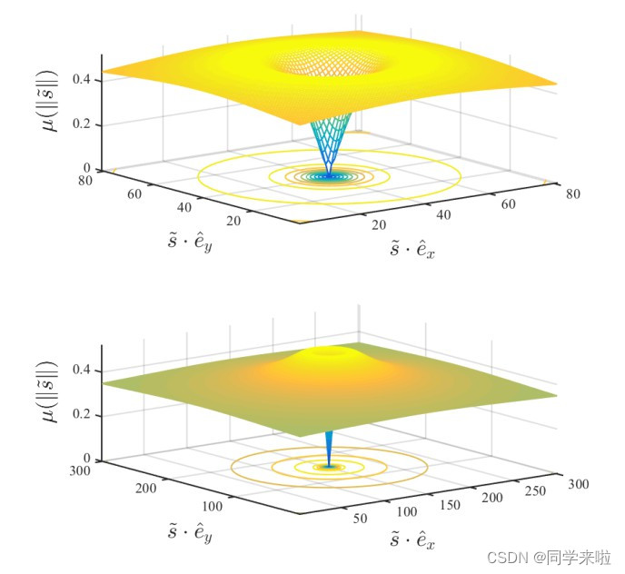
图III.4:顶部的图是放大视图,其描绘了每个轮胎上的车轮滑移到牵引力的映射;底部的图是缩小视图,其重点描绘了定义摩擦圈的峰值。参考方程(III.15)。
The models discussed in this section appear frequently in the literature on motion planning and control for driverless cars. They are suitable for the motion planning and control tasks discussed in this survey. However, lower level control tasks such as electronic stability control and active suspension systems typically use more sophisticated models for the chassis, steering and, drive-train.
本节讨论的模型经常出现在无人驾驶汽车的运动规划和控制的文献中。这些模型适用于本综述所讨论的运动规划和控制任务。然而,诸如电子稳定控制和主动悬架系统等较低级别的控制任务通常使用更复杂的模型来对底盘、转向和传动系统进行建模。


