目录

设置

简介

动机

结构

全局Token创建

模块

窗口

级别

模型

建立模型

预训练权重的理智检查

微调 GCViT 模型

配置

数据加载器

花卉数据集

为花卉数据集重建模型

训练

---

政安晨的个人主页：政安晨

欢迎 👍点赞✍评论⭐收藏

收录专栏: TensorFlow与Keras机器学习实战

希望政安晨的博客能够对您有所裨益，如有不足之处，欢迎在评论区提出指正！

本文目标：用于图像分类的全局上下文视觉变换器的实现和微调。

设置

!pip install --upgrade keras_cv tensorflow
!pip install --upgrade keras

import keras
from keras_cv.layers import DropPath
from keras import ops
from keras import layers

import tensorflow as tf  # only for dataloader
import tensorflow_datasets as tfds  # for flower dataset

from skimage.data import chelsea
import matplotlib.pyplot as plt
import numpy as np

简介

在本文中，我们将利用多后端 Keras 3.0 来实现 A Hatamizadeh 等人在 ICML 2023 上发表的 GCViT：Global Context Vision Transformer 论文，并利用官方 ImageNet 预训练的权重在 Flower 数据集上对模型进行微调，以完成图像分类任务。

本文的一大亮点是与多个后端兼容：TensorFlow、PyTorch 和 JAX，展示了多后端 Keras 的真正潜力。

动机

注：在本文这部分中，我们将了解 GCViT 的背景，并尝试理解提出它的原因。

近年来，变换器在自然语言处理（NLP）任务中占据了主导地位，其自我注意机制可同时捕捉长程和短程信息。
顺应这一趋势，Vision Transformer（ViT）提出在一个类似于原始 Transformer 编码器的巨大架构中利用图像补丁作为标记。
尽管卷积神经网络（CNN）在计算机视觉领域一直占据主导地位，但基于 ViT 的模型已在各种计算机视觉任务中显示出 SOTA 或具有竞争力的性能。

然而，由于自注意的计算复杂度为二次方[O(n^2)]，且缺乏多尺度信息，因此很难将 ViT 视为计算视觉任务（如分割和物体检测）的通用架构，因为它需要在像素级进行密集预测。

Swin Transformer 曾试图通过提出多分辨率/分层架构来解决 ViT 的问题，在这种架构中，自注意力是在局部窗口中计算的，而跨窗口连接（如窗口移动）则用于对不同区域之间的交互进行建模。但局部窗口的感受野有限，无法捕捉长距离信息，而窗口移动等跨窗口连接方案只能覆盖每个窗口附近的小范围邻域。此外，它还缺乏归纳偏差，而归纳偏差鼓励一定的翻译不变性，这对于通用视觉建模，尤其是物体检测和语义分割等密集预测任务来说，仍然是可取的。

针对上述局限性，我们提出了全局语境（GC）ViT 网络。

结构

让我们快速浏览一下我们的关键组件：

1. 干/补丁嵌入层（Stem/PatchEmbed）：干/补丁层在网络开始时处理图像。对于该网络，它创建补丁/标记，并将其转换为嵌入。

2.层（Level）：它是重复性的构建模块，使用不同的模块提取特征。

3.全局令牌生成/特征提取：它利用 Deepthwise-CNN、SqueezeAndExcitation（Squeeze-Excitation）、CNN 和 MaxPooling 生成全局标记/片段。因此，它基本上就是一个特征提取器。

4.块：它是一个重复性模块，用于关注特征并将其投射到某个维度。

1.局部-MSA：局部多头自我关注。

2.Global-MSA：全局多头自我注意。

3.MLP：将向量投射到另一维度的线性层。

5.Downsample/ReduceSize：它与全局令牌生成模块非常相似，但它使用 CNN 而不是 MaxPooling 进行降采样，并增加了层归一化模块。

6.头部：它是负责分类任务的模块。

1.池化：它将 N x 2D 特征转换为 N x 1D 特征。

2.分类器：它处理 N x 1D 个特征，从而对类别做出判断。

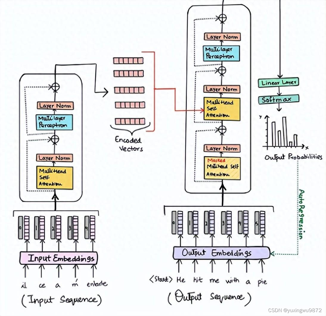
为了便于理解，我对架构图做了注释、

单元模块

注：本模块用于构建本文中的其他模块。大多数模块都是从其他作品中借用的，或者是旧作的修改版。

1.挤压和激发（SqueezeAndExcitation）：挤压-激发（SE）又称瓶颈模块，是一种通道关注。它由 AvgPooling、Dense/FullyConnected（FC）/Linear、GELU 和 Sigmoid 模块组成。

2.Fused-MBConv: 这与 EfficientNetV2 中使用的方法类似。它使用 Depthwise-Conv、GELU、SqueezeAndExcitation 和 Conv 来提取具有重邻关系的特征。需要注意的是，这个模块没有声明新的模块，我们只是直接应用了相应的模块。

3.ReduceSize：这是一个基于 CNN 的降采样模块，其中包括提取特征的 Fused-MBConv 模块、同时降低空间维度和增加通道维度的 Strided Conv 模块，以及对特征进行归一化处理的 LayerNormalization 模块。

在本文/图中，该模块被称为下采样模块。值得一提的是，SwniTransformer 使用了 PatchMerging 模块，而不是 ReduceSize 来减少空间维度和增加通道维度，后者使用的是全连接/密集/线性模块。根据 GCViT 的论文，使用 ReduceSize 的目的之一是通过 CNN 模块增加感应偏置。

4.MLP：这是我们自己的多层感知器模块。这是一个前馈/全连接/线性模块，只需将输入投射到一个任意维度。

class SqueezeAndExcitation(layers.Layer):
    """Squeeze and excitation block.

    Args:
        output_dim: output features dimension, if `None` use same dim as input.
        expansion: expansion ratio.
    """

    def __init__(self, output_dim=None, expansion=0.25, **kwargs):
        super().__init__(**kwargs)
        self.expansion = expansion
        self.output_dim = output_dim

    def build(self, input_shape):
        inp = input_shape[-1]
        self.output_dim = self.output_dim or inp
        self.avg_pool = layers.GlobalAvgPool2D(keepdims=True, name="avg_pool")
        self.fc = [
            layers.Dense(int(inp * self.expansion), use_bias=False, name="fc_0"),
            layers.Activation("gelu", name="fc_1"),
            layers.Dense(self.output_dim, use_bias=False, name="fc_2"),
            layers.Activation("sigmoid", name="fc_3"),
        ]
        super().build(input_shape)

    def call(self, inputs, **kwargs):
        x = self.avg_pool(inputs)
        for layer in self.fc:
            x = layer(x)
        return x * inputs


class ReduceSize(layers.Layer):
    """Down-sampling block.

    Args:
        keepdims: if False spatial dim is reduced and channel dim is increased
    """

    def __init__(self, keepdims=False, **kwargs):
        super().__init__(**kwargs)
        self.keepdims = keepdims

    def build(self, input_shape):
        embed_dim = input_shape[-1]
        dim_out = embed_dim if self.keepdims else 2 * embed_dim
        self.pad1 = layers.ZeroPadding2D(1, name="pad1")
        self.pad2 = layers.ZeroPadding2D(1, name="pad2")
        self.conv = [
            layers.DepthwiseConv2D(
                kernel_size=3, strides=1, padding="valid", use_bias=False, name="conv_0"
            ),
            layers.Activation("gelu", name="conv_1"),
            SqueezeAndExcitation(name="conv_2"),
            layers.Conv2D(
                embed_dim,
                kernel_size=1,
                strides=1,
                padding="valid",
                use_bias=False,
                name="conv_3",
            ),
        ]
        self.reduction = layers.Conv2D(
            dim_out,
            kernel_size=3,
            strides=2,
            padding="valid",
            use_bias=False,
            name="reduction",
        )
        self.norm1 = layers.LayerNormalization(
            -1, 1e-05, name="norm1"
        )  # eps like PyTorch
        self.norm2 = layers.LayerNormalization(-1, 1e-05, name="norm2")

    def call(self, inputs, **kwargs):
        x = self.norm1(inputs)
        xr = self.pad1(x)
        for layer in self.conv:
            xr = layer(xr)
        x = x + xr
        x = self.pad2(x)
        x = self.reduction(x)
        x = self.norm2(x)
        return x


class MLP(layers.Layer):
    """Multi-Layer Perceptron (MLP) block.

    Args:
        hidden_features: hidden features dimension.
        out_features: output features dimension.
        activation: activation function.
        dropout: dropout rate.
    """

    def __init__(
        self,
        hidden_features=None,
        out_features=None,
        activation="gelu",
        dropout=0.0,
        **kwargs,
    ):
        super().__init__(**kwargs)
        self.hidden_features = hidden_features
        self.out_features = out_features
        self.activation = activation
        self.dropout = dropout

    def build(self, input_shape):
        self.in_features = input_shape[-1]
        self.hidden_features = self.hidden_features or self.in_features
        self.out_features = self.out_features or self.in_features
        self.fc1 = layers.Dense(self.hidden_features, name="fc1")
        self.act = layers.Activation(self.activation, name="act")
        self.fc2 = layers.Dense(self.out_features, name="fc2")
        self.drop1 = layers.Dropout(self.dropout, name="drop1")
        self.drop2 = layers.Dropout(self.dropout, name="drop2")

    def call(self, inputs, **kwargs):
        x = self.fc1(inputs)
        x = self.act(x)
        x = self.drop1(x)
        x = self.fc2(x)
        x = self.drop2(x)
        return x

Stem

注释在代码中，该模块被称为 PatchEmbed，但在纸面上，它被称为 Stem。

在模型中，我们首先使用了 patch_embed 模块。让我们试着理解一下这个模块。

从调用方法中我们可以看到：

1.该模块首先对输入进行填充。

2.然后使用卷积提取带有嵌入的补丁。

3.最后，使用 ReduceSize 模块先用卷积提取特征，但既不降低空间维度，也不增加空间维度。

4.值得注意的一点是，与 ViT 或 SwinTransformer 不同，GCViT 会创建重叠的补丁。

我们可以从代码 Conv2D(self.embed_dim, kernel_size=3, strides=2, name='proj') 中发现这一点。如果我们想要不重叠的补丁，就应该使用相同的 kernel_size 和 strides。

5.该模块将输入的空间维度减少了 4 倍。

摘要：图像 → 填充 → 卷积 → （特征提取 + 下采样）

class PatchEmbed(layers.Layer):
    """Patch embedding block.

    Args:
        embed_dim: feature size dimension.
    """

    def __init__(self, embed_dim, **kwargs):
        super().__init__(**kwargs)
        self.embed_dim = embed_dim

    def build(self, input_shape):
        self.pad = layers.ZeroPadding2D(1, name="pad")
        self.proj = layers.Conv2D(self.embed_dim, 3, 2, name="proj")
        self.conv_down = ReduceSize(keepdims=True, name="conv_down")

    def call(self, inputs, **kwargs):
        x = self.pad(inputs)
        x = self.proj(x)
        x = self.conv_down(x)
        return x

全局Token创建

注释它是两个 CNN 模块之一，用于模拟感应偏差。

从上面的单元格中我们可以看到，在这一层中，我们首先使用了 to_q_global/Global Token Gen./FeatureExtraction。

让我们来了解一下它是如何工作的：

× 此模块是 FeatureExtract 模块的系列，根据论文，我们需要重复此模块 K 次，其中 K = log2(H/h)，H = feature_map_height，W = feature_map_width。
× 特征提取：这一层与 ReduceSize 模块非常相似，但它使用 MaxPooling 模块来减少维度，不增加特征维度（channelie），也不使用 LayerNormalizaton。该模块被反复用于 Generate Token Gen. 模块，为全局上下文关注生成全局标记。
×从图中需要注意的一点是，全局标记在整个图像中共享，这意味着我们只使用一个全局窗口来处理图像中的所有局部标记。这使得计算非常高效。
×对于输入形状为（B、H、W、C）的特征图，我们将得到输出形状（B、H、W、C）。如果我们将这些全局标记复制到图像中的 M 个局部窗口，其中 M = (H x W)/(h x w) = num_window，那么输出形状为：（B * M, h, w, C）"。

摘要：该模块用于调整图像大小以适应窗口。

class FeatureExtraction(layers.Layer):
    """Feature extraction block.

    Args:
        keepdims: bool argument for maintaining the resolution.
    """

    def __init__(self, keepdims=False, **kwargs):
        super().__init__(**kwargs)
        self.keepdims = keepdims

    def build(self, input_shape):
        embed_dim = input_shape[-1]
        self.pad1 = layers.ZeroPadding2D(1, name="pad1")
        self.pad2 = layers.ZeroPadding2D(1, name="pad2")
        self.conv = [
            layers.DepthwiseConv2D(3, 1, use_bias=False, name="conv_0"),
            layers.Activation("gelu", name="conv_1"),
            SqueezeAndExcitation(name="conv_2"),
            layers.Conv2D(embed_dim, 1, 1, use_bias=False, name="conv_3"),
        ]
        if not self.keepdims:
            self.pool = layers.MaxPool2D(3, 2, name="pool")
        super().build(input_shape)

    def call(self, inputs, **kwargs):
        x = inputs
        xr = self.pad1(x)
        for layer in self.conv:
            xr = layer(xr)
        x = x + xr
        if not self.keepdims:
            x = self.pool(self.pad2(x))
        return x


class GlobalQueryGenerator(layers.Layer):
    """Global query generator.

    Args:
        keepdims: to keep the dimension of FeatureExtraction layer.
        For instance, repeating log(56/7) = 3 blocks, with input
        window dimension 56 and output window dimension 7 at down-sampling
        ratio 2. Please check Fig.5 of GC ViT paper for details.
    """

    def __init__(self, keepdims=False, **kwargs):
        super().__init__(**kwargs)
        self.keepdims = keepdims

    def build(self, input_shape):
        self.to_q_global = [
            FeatureExtraction(keepdims, name=f"to_q_global_{i}")
            for i, keepdims in enumerate(self.keepdims)
        ]
        super().build(input_shape)

    def call(self, inputs, **kwargs):
        x = inputs
        for layer in self.to_q_global:
            x = layer(x)
        return x

注意事项
这是本文的核心要点。

从调用方法中我们可以看到： WindowAttention 模块会根据 global_query 参数应用本地和全局窗口注意力。
1.首先，它将输入特征转换成查询、键、值，用于局部关注；将键、值转换成键、值，用于全局关注。对于全局关注，它将从全局令牌 Gen 中获取全局查询。qkv = tf.reshape(qkv, [B_, N, self.qkv_size, self.num_heads, C // self.num_heads])
2.在发送查询、键和值以引起注意之前，全局令牌要经过一个重要的过程。q_global = tf.repeat(q_global,repeats=B_//B,axis=0)，这里 B_//B 表示图像中的窗口数。
3.然后根据 global_query 参数，简单地应用局部窗口自注意或全局窗口注意。代码中值得注意的一点是，我们使用注意力掩码添加了相对位置嵌入，而不是补丁嵌入。 attn = attn + relative_position_bias[tf.newaxis,

4.现在，让我们思考一下，试着理解一下这里发生了什么。

请看下图。从左图我们可以看到，在本地注意力模式下，查询是本地的，而且仅限于本地窗口（红色方框），因此我们无法获取远程信息。而在右图中，由于是全局查询，我们现在不再局限于本地窗口（蓝色方框），我们可以获取远距离信息。

5. 在 ViT 中，我们将（注意力）图像图元与图像图元进行比较，在 SwinTransformer 中，我们将窗口图元与窗口图元进行比较，但在 GCViT 中，我们将图像图元与窗口图元进行比较。

但现在您可能会问，即使图像图元的尺寸比窗口图元的尺寸大，又如何比较（关注）图像图元和窗口图元呢？

从上图可以看出，图像图元的形状是（1, 8, 8, 3），而窗口图元的形状是（1, 4, 4, 3））。是的，你说得对，我们无法直接比较它们，因此我们使用全局令牌生成/特征提取 CNN 模块调整了图像令牌的大小，以适应窗口令牌。

下表应该能给您一个清晰的比较：

class WindowAttention(layers.Layer):
    """Local window attention.

    This implementation was proposed by
    [Liu et al., 2021](https://arxiv.org/abs/2103.14030) in SwinTransformer.

    Args:
        window_size: window size.
        num_heads: number of attention head.
        global_query: if the input contains global_query
        qkv_bias: bool argument for query, key, value learnable bias.
        qk_scale: bool argument to scaling query, key.
        attention_dropout: attention dropout rate.
        projection_dropout: output dropout rate.
    """

    def __init__(
        self,
        window_size,
        num_heads,
        global_query,
        qkv_bias=True,
        qk_scale=None,
        attention_dropout=0.0,
        projection_dropout=0.0,
        **kwargs,
    ):
        super().__init__(**kwargs)
        window_size = (window_size, window_size)
        self.window_size = window_size
        self.num_heads = num_heads
        self.global_query = global_query
        self.qkv_bias = qkv_bias
        self.qk_scale = qk_scale
        self.attention_dropout = attention_dropout
        self.projection_dropout = projection_dropout

    def build(self, input_shape):
        embed_dim = input_shape[0][-1]
        head_dim = embed_dim // self.num_heads
        self.scale = self.qk_scale or head_dim**-0.5
        self.qkv_size = 3 - int(self.global_query)
        self.qkv = layers.Dense(
            embed_dim * self.qkv_size, use_bias=self.qkv_bias, name="qkv"
        )
        self.relative_position_bias_table = self.add_weight(
            name="relative_position_bias_table",
            shape=[
                (2 * self.window_size[0] - 1) * (2 * self.window_size[1] - 1),
                self.num_heads,
            ],
            initializer=keras.initializers.TruncatedNormal(stddev=0.02),
            trainable=True,
            dtype=self.dtype,
        )
        self.attn_drop = layers.Dropout(self.attention_dropout, name="attn_drop")
        self.proj = layers.Dense(embed_dim, name="proj")
        self.proj_drop = layers.Dropout(self.projection_dropout, name="proj_drop")
        self.softmax = layers.Activation("softmax", name="softmax")
        super().build(input_shape)

    def get_relative_position_index(self):
        coords_h = ops.arange(self.window_size[0])
        coords_w = ops.arange(self.window_size[1])
        coords = ops.stack(ops.meshgrid(coords_h, coords_w, indexing="ij"), axis=0)
        coords_flatten = ops.reshape(coords, [2, -1])
        relative_coords = coords_flatten[:, :, None] - coords_flatten[:, None, :]
        relative_coords = ops.transpose(relative_coords, axes=[1, 2, 0])
        relative_coords_xx = relative_coords[:, :, 0] + self.window_size[0] - 1
        relative_coords_yy = relative_coords[:, :, 1] + self.window_size[1] - 1
        relative_coords_xx = relative_coords_xx * (2 * self.window_size[1] - 1)
        relative_position_index = relative_coords_xx + relative_coords_yy
        return relative_position_index

    def call(self, inputs, **kwargs):
        if self.global_query:
            inputs, q_global = inputs
            B = ops.shape(q_global)[0]  # B, N, C
        else:
            inputs = inputs[0]
        B_, N, C = ops.shape(inputs)  # B*num_window, num_tokens, channels
        qkv = self.qkv(inputs)
        qkv = ops.reshape(
            qkv, [B_, N, self.qkv_size, self.num_heads, C // self.num_heads]
        )
        qkv = ops.transpose(qkv, [2, 0, 3, 1, 4])
        if self.global_query:
            k, v = ops.split(
                qkv, indices_or_sections=2, axis=0
            )  # for unknown shame num=None will throw error
            q_global = ops.repeat(
                q_global, repeats=B_ // B, axis=0
            )  # num_windows = B_//B => q_global same for all windows in a img
            q = ops.reshape(q_global, [B_, N, self.num_heads, C // self.num_heads])
            q = ops.transpose(q, axes=[0, 2, 1, 3])
        else:
            q, k, v = ops.split(qkv, indices_or_sections=3, axis=0)
            q = ops.squeeze(q, axis=0)

        k = ops.squeeze(k, axis=0)
        v = ops.squeeze(v, axis=0)

        q = q * self.scale
        attn = q @ ops.transpose(k, axes=[0, 1, 3, 2])
        relative_position_bias = ops.take(
            self.relative_position_bias_table,
            ops.reshape(self.get_relative_position_index(), [-1]),
        )
        relative_position_bias = ops.reshape(
            relative_position_bias,
            [
                self.window_size[0] * self.window_size[1],
                self.window_size[0] * self.window_size[1],
                -1,
            ],
        )
        relative_position_bias = ops.transpose(relative_position_bias, axes=[2, 0, 1])
        attn = attn + relative_position_bias[None,]
        attn = self.softmax(attn)
        attn = self.attn_drop(attn)

        x = ops.transpose((attn @ v), axes=[0, 2, 1, 3])
        x = ops.reshape(x, [B_, N, C])
        x = self.proj_drop(self.proj(x))
        return x

模块

备注：该模块没有任何卷积模块。

在本级别中，我们使用的第二个模块是块。让我们来了解一下它是如何工作的。

从调用方法中我们可以看到：

1.Block 模块只接受用于局部关注的 feature_maps，或者接受用于全局关注的附加全局查询。

2. 在发送用于关注的特征图之前，该模块会将批量特征图转换为批量窗口，因为我们将应用窗口关注。

3. 然后，我们将批量发送批量窗口以供关注。

4. 应用注意力后，我们将批量窗口还原为批量特征图。

5. 在将注意力发送到应用特征输出之前，该模块会在残差连接中应用随机深度正则化。

此外，在应用随机深度正则化之前，它还会使用可训练参数对输入进行重新缩放。

需要注意的是，随机深度模块并没有在本文的图中显示。

窗口

在图块模块中，我们在应用注意力前后创建了窗口。下面的模块将特征图（B、H、W、C）转换为堆叠窗口（B x H/h x W/w、h、w、C）→（num_windows_batch、window_size、window_size、channel） * 该模块使用重塑和转置（reshape & transpose）从图像中创建这些窗口，而不是对它们进行迭代。

class Block(layers.Layer):
    """GCViT block.

    Args:
        window_size: window size.
        num_heads: number of attention head.
        global_query: apply global window attention
        mlp_ratio: MLP ratio.
        qkv_bias: bool argument for query, key, value learnable bias.
        qk_scale: bool argument to scaling query, key.
        drop: dropout rate.
        attention_dropout: attention dropout rate.
        path_drop: drop path rate.
        activation: activation function.
        layer_scale: layer scaling coefficient.
    """

    def __init__(
        self,
        window_size,
        num_heads,
        global_query,
        mlp_ratio=4.0,
        qkv_bias=True,
        qk_scale=None,
        dropout=0.0,
        attention_dropout=0.0,
        path_drop=0.0,
        activation="gelu",
        layer_scale=None,
        **kwargs,
    ):
        super().__init__(**kwargs)
        self.window_size = window_size
        self.num_heads = num_heads
        self.global_query = global_query
        self.mlp_ratio = mlp_ratio
        self.qkv_bias = qkv_bias
        self.qk_scale = qk_scale
        self.dropout = dropout
        self.attention_dropout = attention_dropout
        self.path_drop = path_drop
        self.activation = activation
        self.layer_scale = layer_scale

    def build(self, input_shape):
        B, H, W, C = input_shape[0]
        self.norm1 = layers.LayerNormalization(-1, 1e-05, name="norm1")
        self.attn = WindowAttention(
            window_size=self.window_size,
            num_heads=self.num_heads,
            global_query=self.global_query,
            qkv_bias=self.qkv_bias,
            qk_scale=self.qk_scale,
            attention_dropout=self.attention_dropout,
            projection_dropout=self.dropout,
            name="attn",
        )
        self.drop_path1 = DropPath(self.path_drop)
        self.drop_path2 = DropPath(self.path_drop)
        self.norm2 = layers.LayerNormalization(-1, 1e-05, name="norm2")
        self.mlp = MLP(
            hidden_features=int(C * self.mlp_ratio),
            dropout=self.dropout,
            activation=self.activation,
            name="mlp",
        )
        if self.layer_scale is not None:
            self.gamma1 = self.add_weight(
                name="gamma1",
                shape=[C],
                initializer=keras.initializers.Constant(self.layer_scale),
                trainable=True,
                dtype=self.dtype,
            )
            self.gamma2 = self.add_weight(
                name="gamma2",
                shape=[C],
                initializer=keras.initializers.Constant(self.layer_scale),
                trainable=True,
                dtype=self.dtype,
            )
        else:
            self.gamma1 = 1.0
            self.gamma2 = 1.0
        self.num_windows = int(H // self.window_size) * int(W // self.window_size)
        super().build(input_shape)

    def call(self, inputs, **kwargs):
        if self.global_query:
            inputs, q_global = inputs
        else:
            inputs = inputs[0]
        B, H, W, C = ops.shape(inputs)
        x = self.norm1(inputs)
        # create windows and concat them in batch axis
        x = self.window_partition(x, self.window_size)  # (B_, win_h, win_w, C)
        # flatten patch
        x = ops.reshape(x, [-1, self.window_size * self.window_size, C])
        # attention
        if self.global_query:
            x = self.attn([x, q_global])
        else:
            x = self.attn([x])
        # reverse window partition
        x = self.window_reverse(x, self.window_size, H, W, C)
        # FFN
        x = inputs + self.drop_path1(x * self.gamma1)
        x = x + self.drop_path2(self.gamma2 * self.mlp(self.norm2(x)))
        return x

    def window_partition(self, x, window_size):
        """
        Args:
            x: (B, H, W, C)
            window_size: window size
        Returns:
            local window features (num_windows*B, window_size, window_size, C)
        """
        B, H, W, C = ops.shape(x)
        x = ops.reshape(
            x,
            [
                -1,
                H // window_size,
                window_size,
                W // window_size,
                window_size,
                C,
            ],
        )
        x = ops.transpose(x, axes=[0, 1, 3, 2, 4, 5])
        windows = ops.reshape(x, [-1, window_size, window_size, C])
        return windows

    def window_reverse(self, windows, window_size, H, W, C):
        """
        Args:
            windows: local window features (num_windows*B, window_size, window_size, C)
            window_size: Window size
            H: Height of image
            W: Width of image
            C: Channel of image
        Returns:
            x: (B, H, W, C)
        """
        x = ops.reshape(
            windows,
            [
                -1,
                H // window_size,
                W // window_size,
                window_size,
                window_size,
                C,
            ],
        )
        x = ops.transpose(x, axes=[0, 1, 3, 2, 4, 5])
        x = ops.reshape(x, [-1, H, W, C])
        return x

级别

注：该模块包含变压器模块和 CNN 模块。

在模型中，我们使用的第二个模块是 Level。让我们试着理解一下这个模块。从调用方法中我们可以看到：

1.首先，它创建了带有一系列特征提取模块的 global_token。稍后我们会看到，FeatureExtraction 只是一个基于 CNN 的简单模块。

2. 然后，它使用一系列的 Block 模块，根据深度级别应用局部或全局窗口注意力。

3. 最后，它使用 ReduceSize 缩减上下文特征的维度。

摘要： feature_map → global_token → local/lobal window attention → dowsample

class Level(layers.Layer):
    """GCViT level.

    Args:
        depth: number of layers in each stage.
        num_heads: number of heads in each stage.
        window_size: window size in each stage.
        keepdims: dims to keep in FeatureExtraction.
        downsample: bool argument for down-sampling.
        mlp_ratio: MLP ratio.
        qkv_bias: bool argument for query, key, value learnable bias.
        qk_scale: bool argument to scaling query, key.
        drop: dropout rate.
        attention_dropout: attention dropout rate.
        path_drop: drop path rate.
        layer_scale: layer scaling coefficient.
    """

    def __init__(
        self,
        depth,
        num_heads,
        window_size,
        keepdims,
        downsample=True,
        mlp_ratio=4.0,
        qkv_bias=True,
        qk_scale=None,
        dropout=0.0,
        attention_dropout=0.0,
        path_drop=0.0,
        layer_scale=None,
        **kwargs,
    ):
        super().__init__(**kwargs)
        self.depth = depth
        self.num_heads = num_heads
        self.window_size = window_size
        self.keepdims = keepdims
        self.downsample = downsample
        self.mlp_ratio = mlp_ratio
        self.qkv_bias = qkv_bias
        self.qk_scale = qk_scale
        self.dropout = dropout
        self.attention_dropout = attention_dropout
        self.path_drop = path_drop
        self.layer_scale = layer_scale

    def build(self, input_shape):
        path_drop = (
            [self.path_drop] * self.depth
            if not isinstance(self.path_drop, list)
            else self.path_drop
        )
        self.blocks = [
            Block(
                window_size=self.window_size,
                num_heads=self.num_heads,
                global_query=bool(i % 2),
                mlp_ratio=self.mlp_ratio,
                qkv_bias=self.qkv_bias,
                qk_scale=self.qk_scale,
                dropout=self.dropout,
                attention_dropout=self.attention_dropout,
                path_drop=path_drop[i],
                layer_scale=self.layer_scale,
                name=f"blocks_{i}",
            )
            for i in range(self.depth)
        ]
        self.down = ReduceSize(keepdims=False, name="downsample")
        self.q_global_gen = GlobalQueryGenerator(self.keepdims, name="q_global_gen")
        super().build(input_shape)

    def call(self, inputs, **kwargs):
        x = inputs
        q_global = self.q_global_gen(x)  # shape: (B, win_size, win_size, C)
        for i, blk in enumerate(self.blocks):
            if i % 2:
                x = blk([x, q_global])  # shape: (B, H, W, C)
            else:
                x = blk([x])  # shape: (B, H, W, C)
        if self.downsample:
            x = self.down(x)  # shape: (B, H//2, W//2, 2*C)
        return x

模型

让我们直接跳转到模型。从调用方法中我们可以看到：

1.它从图像中创建补丁嵌入。这一层不会对这些嵌入式进行扁平化处理，这意味着该模块的输出将是（batch, height/window_size, width/window_size, embed_dim），而不是（batch, height x width/window_size^2, embed_dim）。

2. 将这些嵌入信息传递给一系列 Level 模块，我们称之为 Level，其中包括：

× 生成全局标记

× 应用局部和全局注意力

× 最后应用降采样。

3.因此，经过 n 层后的输出形状为：（batch, width/window_size x 2^{n-1}, width/window_size x 2^{n-1}, embed_dim x 2^{n-1}）。

在最后一层，本文不使用降采样和增加通道。

4.使用 LayerNormalization 模块对上述层的输出进行归一化处理。

5.在头部，使用池化模块将二维特征转换为一维特征。该模块之后的输出形状为（batch, embed_dim x 2^{n-1}）。

最后，池化后的特征被发送到 Dense/Linear 模块进行分类。

总和：图像 → （补丁 + 嵌入） → 剔除 → （注意 + 特征提取） → 归一化 → 汇集 → 分类

class GCViT(keras.Model):
    """GCViT model.

    Args:
        window_size: window size in each stage.
        embed_dim: feature size dimension.
        depths: number of layers in each stage.
        num_heads: number of heads in each stage.
        drop_rate: dropout rate.
        mlp_ratio: MLP ratio.
        qkv_bias: bool argument for query, key, value learnable bias.
        qk_scale: bool argument to scaling query, key.
        attention_dropout: attention dropout rate.
        path_drop: drop path rate.
        layer_scale: layer scaling coefficient.
        num_classes: number of classes.
        head_activation: activation function for head.
    """

    def __init__(
        self,
        window_size,
        embed_dim,
        depths,
        num_heads,
        drop_rate=0.0,
        mlp_ratio=3.0,
        qkv_bias=True,
        qk_scale=None,
        attention_dropout=0.0,
        path_drop=0.1,
        layer_scale=None,
        num_classes=1000,
        head_activation="softmax",
        **kwargs,
    ):
        super().__init__(**kwargs)
        self.window_size = window_size
        self.embed_dim = embed_dim
        self.depths = depths
        self.num_heads = num_heads
        self.drop_rate = drop_rate
        self.mlp_ratio = mlp_ratio
        self.qkv_bias = qkv_bias
        self.qk_scale = qk_scale
        self.attention_dropout = attention_dropout
        self.path_drop = path_drop
        self.layer_scale = layer_scale
        self.num_classes = num_classes
        self.head_activation = head_activation

        self.patch_embed = PatchEmbed(embed_dim=embed_dim, name="patch_embed")
        self.pos_drop = layers.Dropout(drop_rate, name="pos_drop")
        path_drops = np.linspace(0.0, path_drop, sum(depths))
        keepdims = [(0, 0, 0), (0, 0), (1,), (1,)]
        self.levels = []
        for i in range(len(depths)):
            path_drop = path_drops[sum(depths[:i]) : sum(depths[: i + 1])].tolist()
            level = Level(
                depth=depths[i],
                num_heads=num_heads[i],
                window_size=window_size[i],
                keepdims=keepdims[i],
                downsample=(i < len(depths) - 1),
                mlp_ratio=mlp_ratio,
                qkv_bias=qkv_bias,
                qk_scale=qk_scale,
                dropout=drop_rate,
                attention_dropout=attention_dropout,
                path_drop=path_drop,
                layer_scale=layer_scale,
                name=f"levels_{i}",
            )
            self.levels.append(level)
        self.norm = layers.LayerNormalization(axis=-1, epsilon=1e-05, name="norm")
        self.pool = layers.GlobalAvgPool2D(name="pool")
        self.head = layers.Dense(num_classes, name="head", activation=head_activation)

    def build(self, input_shape):
        super().build(input_shape)
        self.built = True

    def call(self, inputs, **kwargs):
        x = self.patch_embed(inputs)  # shape: (B, H, W, C)
        x = self.pos_drop(x)
        for level in self.levels:
            x = level(x)  # shape: (B, H_, W_, C_)
        x = self.norm(x)
        x = self.pool(x)  # shape: (B, C__)
        x = self.head(x)
        return x

    def build_graph(self, input_shape=(224, 224, 3)):
        """
        ref: https://www.kaggle.com/code/ipythonx/tf-hybrid-efficientnet-swin-transformer-gradcam
        """
        x = keras.Input(shape=input_shape)
        return keras.Model(inputs=[x], outputs=self.call(x), name=self.name)

    def summary(self, input_shape=(224, 224, 3)):
        return self.build_graph(input_shape).summary()

建立模型

让我们用上面介绍的所有模块建立一个完整的模型。

我们将按照论文中提到的配置建立 GCViT-XXTiny 模型。
此外，我们还将加载移植的官方预训练权重，并尝试进行一些预测。

# Model Configs
config = {
    "window_size": (7, 7, 14, 7),
    "embed_dim": 64,
    "depths": (2, 2, 6, 2),
    "num_heads": (2, 4, 8, 16),
    "mlp_ratio": 3.0,
    "path_drop": 0.2,
}
ckpt_link = (
    "https://github.com/awsaf49/gcvit-tf/releases/download/v1.1.6/gcvitxxtiny.keras"
)

# Build Model
model = GCViT(**config)
inp = ops.array(np.random.uniform(size=(1, 224, 224, 3)))
out = model(inp)

# Load Weights
ckpt_path = keras.utils.get_file(ckpt_link.split("/")[-1], ckpt_link)
model.load_weights(ckpt_path)

# Summary
model.summary((224, 224, 3))

执行：

Downloading data from https://github.com/awsaf49/gcvit-tf/releases/download/v1.1.6/gcvitxxtiny.keras
 48767519/48767519 ━━━━━━━━━━━━━━━━━━━━ 0s 0us/step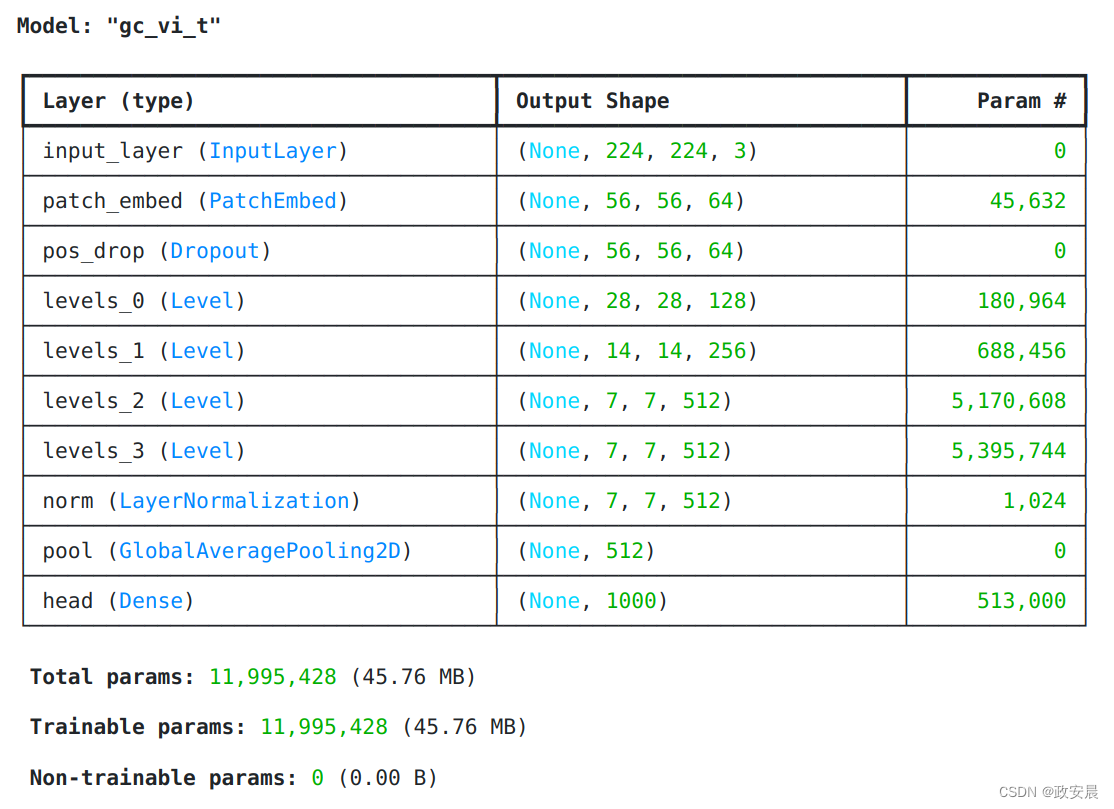

预训练权重的理智检查

img = keras.applications.imagenet_utils.preprocess_input(
    chelsea(), mode="torch"
)  # Chelsea the cat
img = ops.image.resize(img, (224, 224))[None,]  # resize & create batch
pred = model(img)
pred_dec = keras.applications.imagenet_utils.decode_predictions(pred)[0]

print("\n# Image:")
plt.figure(figsize=(6, 6))
plt.imshow(chelsea())
plt.show()
print()

print("# Prediction (Top 5):")
for i in range(5):
    print("{:<12} : {:0.2f}".format(pred_dec[i][1], pred_dec[i][2]))

执行：

Downloading data from https://storage.googleapis.com/download.tensorflow.org/data/imagenet_class_index.json
 35363/35363 ━━━━━━━━━━━━━━━━━━━━ 0s 0us/step

微调 GCViT 模型

在接下来的单元中，我们将在包含 104 个类别的花朵数据集上对 GCViT 模型进行微调。

配置

# Model
IMAGE_SIZE = (224, 224)

# Hyper Params
BATCH_SIZE = 32
EPOCHS = 5

# Dataset
CLASSES = [
    "dandelion",
    "daisy",
    "tulips",
    "sunflowers",
    "roses",
]  # don't change the order

# Other constants
MEAN = 255 * np.array([0.485, 0.456, 0.406], dtype="float32")  # imagenet mean
STD = 255 * np.array([0.229, 0.224, 0.225], dtype="float32")  # imagenet std
AUTO = tf.data.AUTOTUNE

数据加载器

def make_dataset(dataset: tf.data.Dataset, train: bool, image_size: int = IMAGE_SIZE):
    def preprocess(image, label):
        # for training, do augmentation
        if train:
            if tf.random.uniform(shape=[]) > 0.5:
                image = tf.image.flip_left_right(image)
        image = tf.image.resize(image, size=image_size, method="bicubic")
        image = (image - MEAN) / STD  # normalization
        return image, label

    if train:
        dataset = dataset.shuffle(BATCH_SIZE * 10)

    return dataset.map(preprocess, AUTO).batch(BATCH_SIZE).prefetch(AUTO)

花卉数据集

train_dataset, val_dataset = tfds.load(
    "tf_flowers",
    split=["train[:90%]", "train[90%:]"],
    as_supervised=True,
    try_gcs=False,  # gcs_path is necessary for tpu,
)

train_dataset = make_dataset(train_dataset, True)
val_dataset = make_dataset(val_dataset, False)

Downloading and preparing dataset 218.21 MiB (download: 218.21 MiB, generated: 221.83 MiB, total: 440.05 MiB) to /root/tensorflow_datasets/tf_flowers/3.0.1...

Dl Completed...:   0%|          | 0/5 [00:00<?, ? file/s]

Dataset tf_flowers downloaded and prepared to /root/tensorflow_datasets/tf_flowers/3.0.1. Subsequent calls will reuse this data.

为花卉数据集重建模型

# Re-Build Model
model = GCViT(**config, num_classes=104)
inp = ops.array(np.random.uniform(size=(1, 224, 224, 3)))
out = model(inp)

# Load Weights
ckpt_path = keras.utils.get_file(ckpt_link.split("/")[-1], ckpt_link)
model.load_weights(ckpt_path, skip_mismatch=True)

model.compile(
    loss="sparse_categorical_crossentropy", optimizer="adam", metrics=["accuracy"]
)

演绎展示：

/usr/local/lib/python3.10/dist-packages/keras/src/saving/saving_lib.py:269: UserWarning: A total of 1 objects could not be loaded. Example error message for object <Dense name=head, built=True>:

Layer 'head' expected 2 variables, but received 0 variables during loading. Expected: ['kernel', 'bias']

List of objects that could not be loaded:
[<Dense name=head, built=True>]
  warnings.warn(msg)

训练

Epoch 1/5
 104/104 ━━━━━━━━━━━━━━━━━━━━ 153s 581ms/step - accuracy: 0.5140 - loss: 1.4615 - val_accuracy: 0.8828 - val_loss: 0.3485
Epoch 2/5
 104/104 ━━━━━━━━━━━━━━━━━━━━ 7s 69ms/step - accuracy: 0.8775 - loss: 0.3437 - val_accuracy: 0.8828 - val_loss: 0.3508
Epoch 3/5
 104/104 ━━━━━━━━━━━━━━━━━━━━ 7s 68ms/step - accuracy: 0.8937 - loss: 0.2918 - val_accuracy: 0.9019 - val_loss: 0.2953
Epoch 4/5
 104/104 ━━━━━━━━━━━━━━━━━━━━ 7s 68ms/step - accuracy: 0.9232 - loss: 0.2397 - val_accuracy: 0.9183 - val_loss: 0.2212
Epoch 5/5
 104/104 ━━━━━━━━━━━━━━━━━━━━ 7s 68ms/step - accuracy: 0.9456 - loss: 0.1645 - val_accuracy: 0.9210 - val_loss: 0.2897

---