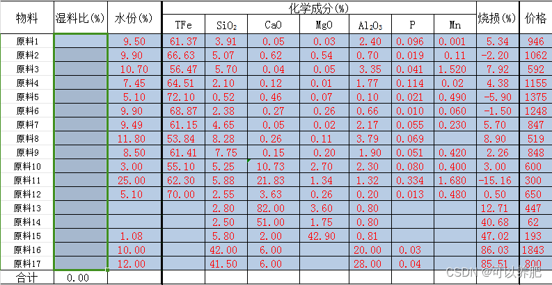
1、工业场景
从很多种铁矿石中选出适合烧结配料的部分铁矿石及其比例,并使其成本最低。
2、数学模型
设Pi代表了第i种原料的成本,xi代表了第i种原料在总配料中的比例,其中i取值为1,2,…,n。计算1吨配料成本:
第种原料的成本是Yi=Pixi1,总成本是Y=∑Yi=∑Pixi,其中i取值为1,2,…,n。目标函数即为:
minY = ∑Yi=∑Pixi
3、使用函数
Scipy.optimize.linprog
def linprog(c, A_ub=None, b_ub=None, A_eq=None, b_eq=None,
            bounds=None, method='interior-point', callback=None,
            options=None, x0=None):
 Parameters
    ----------
    c : 1-D array
        The coefficients of the linear objective function to be minimized.
    A_ub : 2-D array, optional
        The inequality constraint matrix. Each row of ``A_ub`` specifies the
        coefficients of a linear inequality constraint on ``x``.
    b_ub : 1-D array, optional
        The inequality constraint vector. Each element represents an
        upper bound on the corresponding value of ``A_ub @ x``.
    A_eq : 2-D array, optional
        The equality constraint matrix. Each row of ``A_eq`` specifies the
        coefficients of a linear equality constraint on ``x``.
    b_eq : 1-D array, optional
        The equality constraint vector. Each element of ``A_eq @ x`` must equal
        the corresponding element of ``b_eq``.
    bounds : sequence, optional
        A sequence of ``(min, max)`` pairs for each element in ``x``, defining
        the minimum and maximum values of that decision variable. Use ``None``
        to indicate that there is no bound. By default, bounds are
        ``(0, None)`` (all decision variables are non-negative).
        If a single tuple ``(min, max)`` is provided, then ``min`` and
        ``max`` will serve as bounds for all decision variables.
c 目标函数的决策变量对应的系数向量
在这里也就是由17种原料的每吨成本价格构成的向量
A_ub 不等式约束组成的决策变量系数矩阵
在这里也就是17种原料的每种化学成分构成的向量
b_ub 由A_ub对应不等式顺序的阈值向量
在这里也就是每种化学成分对应烧结矿的影响
A_eq	等式约束组成的决策变量系数矩阵
b_eq	由A_ub对应等式顺序的阈值向量
这一组是等式约束,在这里17种原料的比例之和等于1
bounds 表示决策变量x连续的定义域的n×2维矩阵,None表示无穷
这里表示的是对应17种原料的控制范围最小值最大值,是一个n×2维矩阵,n为原料的个数17,
method	调用的求解方法
callback	选择的回调函数
options	求解器选择的字典
x0	初始假设的决策变量向量,若可行linprog会对方法优化
4、代码
from scipy.optimize import linprog
import numpy as np

c=np.array([946,1062,592,1155,1375,1248,847,519,848,600,300,650,447,62,193,1843,800]).transpose()
A_ub = np.array([
                [0.6137, 0.6663, 0.5647, 0.6451, 0.7210, 0.6887, 0.6115, 0.5384, 0.6141, 0.5510, 0.6230, 0.7000, 0.00, 0.00, 0.00, 0.00, 0.00],
                [-0.6137, -0.6663, -0.5647, -0.6451, -0.7210, -0.6887, -0.6115, -0.5384, -0.6141, -0.5510, -0.6230, -0.7000, -0.00, -0.00, -0.00, -0.00, -0.00],
                [0.0391,0.0507 ,0.0570,0.0210 ,0.0052 ,0.0238 ,0.0465 ,0.0828 ,0.0775,0.0525 ,0.0588 ,0.0255 ,0.0280 ,0.0250 ,0.0580 ,0.4200 ,0.4150 ],
                [-0.0391,-0.0507 ,-0.0570,-0.0210 ,-0.0052 ,-0.0238 ,-0.0465 ,-0.0828 ,-0.0775,-0.0525 ,-0.0588 ,-0.0255 ,-0.0280 ,-0.0250 ,-0.0580 ,-0.4200 ,-0.4150 ],
                [0.0003,0.0054 ,0.0005,0.0001 ,0.0007 ,0.0026,0.0002,0.0011 ,0.0020,0.0270 ,0.0134 ,0.0026 ,0.0360 ,0.0175 ,0.4290 ,0.00 ,0.00 ],
                [-0.0003,-0.0054 ,-0.0005,-0.0001 ,-0.0007 ,-0.0026,-0.0002,-0.0011 ,-0.0020,-0.0270 ,-0.0134 ,-0.0026 ,-0.0360 ,-0.0175 ,-0.4290 ,-0.00 ,-0.00 ],
                [0.0240,0.0070 ,0.0335,0.0177 ,0.0010 ,0.0066 ,0.0217 ,0.0379 ,0.0190,0.0230 ,0.0132 ,0.0020 ,0.0080 ,0.0080 ,0.0081 ,0.2000 ,0.2800 ],
                [-0.0240,-0.0070 ,-0.0335,-0.0177 ,-0.0010 ,-0.0066 ,-0.0217 ,-0.0379 ,-0.0190,-0.0230 ,-0.0132 ,-0.0020 ,-0.0080 ,-0.0080 ,-0.0081 ,-0.2000 ,-0.2800 ],
                [0.00096 ,0.00019 ,0.00041 ,0.00114 ,0.00021 ,0.00010 ,0.00055 ,0.00069 ,0.00051 ,0.00080 ,0.00334 ,0.00013 ,0.00 ,0.00 ,0.00 ,0.0003 ,0.0004 ],
                [-0.00096 ,-0.00019 ,-0.00041 ,-0.00114 ,-0.00021 ,-0.00010 ,-0.00055 ,-0.00069 ,-0.00051 ,-0.00080 ,-0.00334 ,-0.00013 ,-0.00 ,-0.00 ,-0.00 ,-0.0003 ,-0.0004 ],
                [0.00001 ,0.0011,0.01520 ,0.0002 ,0.00490 ,0.00060 ,0.00230 ,0.000 ,0.00420 ,0.00400 ,0.01680 ,0.00480 ,0.00 ,0.00 ,0.00 ,0.00 ,0.00 ],
                [-0.00001 ,-0.0011,-0.01520 ,-0.0002 ,-0.00490 ,-0.00060 ,-0.00230 ,-0.000 ,-0.00420 ,-0.00400 ,-0.01680 ,-0.00480 ,-0.00 ,-0.00 ,-0.00 ,-0.00 ,-0.00]])
b_ub = np.array([57,-55,7,-4,3.5,-1.5,3,-1.5,1.1,-0.04,0.7,-0.2])

A_eq = np.array([[1,1,1,1,1,1,1,1,1,1,1,1,1,1,1,1,1]])
b_eq = np.array([100])

x=linprog(c,A_ub,b_ub,A_eq,b_eq,method='highs',bounds=np.array([[10,20],[1,10],[1,10],[1,10],[1,10],[1,10],[1,10],[1,10],[10,20],[10,20],[0,1],[0,2],[5,8],[0,2],[3,5],[3,5],[0.5,2]]))
print(x)
5、计算结果
           con: array([0.])
 crossover_nit: 0
         eqlin:  marginals: array([-2092.4011976])
  residual: array([0.])
           fun: 86687.33832335332
       ineqlin:  marginals: array([   -0.       , -4850.2994012,    -0.       ,    -0.       ,
          -0.       ,    -0.       ,    -0.       ,    -0.       ,
          -0.       ,    -0.       ,    -0.       ,    -0.       ])
  residual: array([2.        , 0.        , 0.7905684 , 2.2094316 , 1.62490589,
       0.37509411, 0.58011713, 0.91988287, 1.05100968, 0.00899032,
       0.31292236, 0.18707764])
         lower:  marginals: <MemoryView of 'ndarray' at 0xb0686e8>
  residual: array([ 0.        ,  9.        ,  9.        ,  0.        ,  9.        ,
        1.29607452,  9.        ,  1.20392548, 10.        ,  0.        ,
        1.        ,  2.        ,  0.        ,  0.        ,  0.        ,
        0.        ,  0.        ])
       message: 'Optimization terminated successfully.'
           nit: 9
         slack: array([2.        , 0.        , 0.7905684 , 2.2094316 , 1.62490589,
       0.37509411, 0.58011713, 0.91988287, 1.05100968, 0.00899032,
       0.31292236, 0.18707764])
        status: 0
       success: True
         upper:  marginals: <MemoryView of 'ndarray' at 0xb068540>
  residual: array([10.        ,  0.        ,  0.        ,  9.        ,  0.        ,
        7.70392548,  0.        ,  7.79607452,  0.        , 10.        ,
        0.        ,  0.        ,  3.        ,  2.        ,  2.        ,
        2.        ,  1.5       ])
             x: array([10.        , 10.        , 10.        ,  1.        , 10.        ,
        2.29607452, 10.        ,  2.20392548, 20.        , 10.        ,
        1.        ,  2.        ,  5.        ,  0.        ,  3.        ,
        3.        ,  0.5       ])

Process finished with exit code 0
最后的x: array就是我们想要的值
[10., 10., 10., 1., 10.,2.29607452, 10., 2.20392548, 20., 10.,1., 2., 5., 0., 3.,3., 0.5]
6、带入实际验证公式
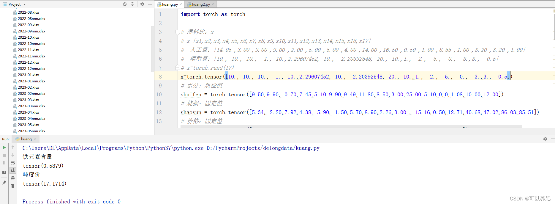
铁元素含量
tensor(0.5879)
吨度价
tensor(17.1714)
7、同一批料对比人工测算
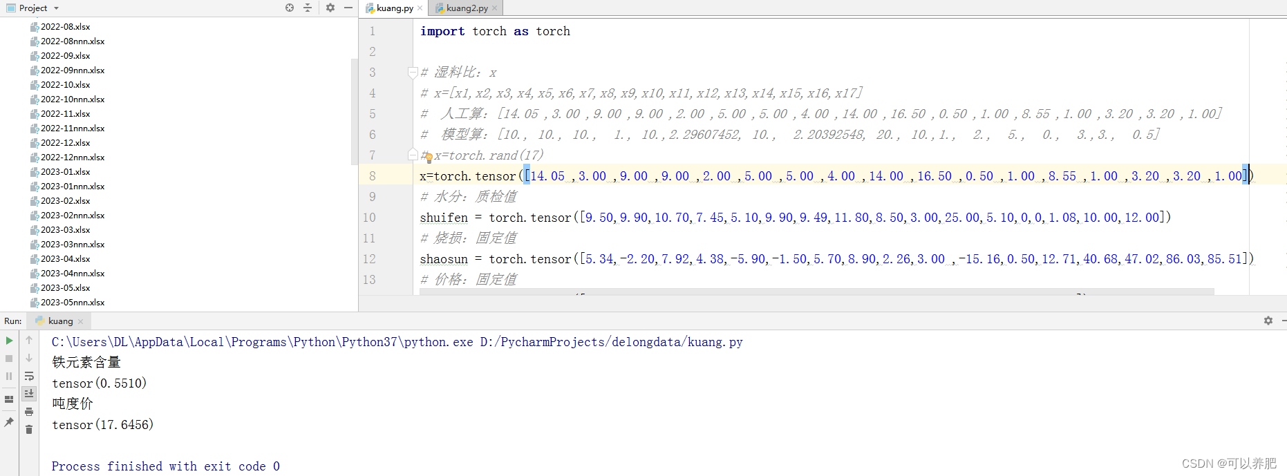 铁元素含量
铁元素含量
tensor(0.5510)
吨度价
tensor(17.6456)
