一、本文介绍
本文介绍的内容是在时间序列中异常值处理的方法,当我进行时间序列分析建模收集数据的过程中,往往都存在着一些特数据情况导致数据中存在着一些异常值,这些异常值往往会导致模型识别到不正常的模式从而无法准确的预测, (我试验过一个数据集清楚之后MAE的精度甚至能提升0.1左右),所以对于异常值的检测和处理对于时间序列来说是十分重要的,本篇文章需要配合我的另一篇文章配合阅读,另一篇文章介绍了如何进行异常值检测,所以本文篇文章下面来介绍当我们检测出异常值之后如何进行异常值处理。
前文回顾:时间序列预测:深度学习、机器学习、融合模型、创新模型实战案例
目录
一、本文介绍
二、异常值处理的方法
三、数据集介绍
四、异常值处理
4.1 删除法
4.2 替换法
4.2.1 平均值替换
4.2.2 中位数替换
4.2.3 众数替换
4.2.4 移动平滑替换
4.3 变换法
4.3.1 Box-Cox变化
4.3.2 对数变化
4.4 分箱法
4.5 使用机器学习模型
4.6 基于规则的方法
五、全文总结
二、异常值处理的方法
处理异常值,主要有以下几种方法:
删除法:直接删除含有异常值的数据。这种方法简单直接,但可能会丢失其他有用信息。
替换法:
- 平均值替换:用整个数据集的平均值替换异常值。
- 中位数替换:用中位数来替换异常值,尤其适用于数据不对称分布的情况。
- 众数替换:对于分类数据,可以使用众数来替换异常值。
- 平滑窗口替换:用异常值附近的平均值替换,需要设定一个窗口大小
变换法:
- 对数变换:适用于右偏数据,可以减少数据的偏斜。
- Box-Cox变换:一种通用的转换方法,可以处理各种类型的偏态分布。
分箱法:将数据分成几个区间(箱子),然后用箱子的边界值或中值来替换异常值。
使用机器学习模型:通过构建模型预测异常值并替换。这种方法通常在数据量较大且复杂时使用。
基于规则的方法:根据领域知识或特定规则来确定和处理异常值。
总结:选择哪种方法取决于异常值的性质和分析的目标。在某些情况下,结合使用多种方法可能会更有效。例如,可以先通过替换或修正方法处理异常值,然后使用变换或鲁棒性较强的模型进行分析。重要的是要理解异常值的来源和它们对分析结果可能产生的影响,从而做出恰当的处理。
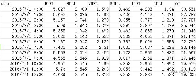
三、数据集介绍
我们本文用到的数据集是官方的ETTh1.csv ,该数据集是一个用于时间序列预测的电力负荷数据集,它是 ETTh 数据集系列中的一个。ETTh 数据集系列通常用于测试和评估时间序列预测模型。以下是 ETTh1.csv 数据集的一些内容:
数据内容:该数据集通常包含有关电力系统的多种变量,如电力负荷、天气情况等。这些变量可以用于预测未来的电力需求或价格。
时间范围和分辨率:数据通常按小时或天记录,涵盖了数月或数年的时间跨度。具体的时间范围和分辨率可能会根据数据集的版本而异。
以下是该数据集的部分截图->
四、异常值处理
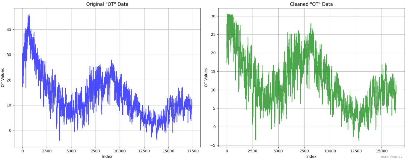
4.1 删除法
删除法:直接删除含有异常值的数据。这种方法简单直接,但可能会丢失其他有用信息。
推荐指数:⭐
import pandas as pd
from scipy.stats import zscore
import matplotlib.pyplot as plt

# Load the data
file_path = 'ETTh1.csv'  # Replace with your file path
data = pd.read_csv(file_path)

# Calculate Z-Scores for the 'OT' column
data['OT_ZScore'] = zscore(data['OT'])

# Filter out rows where the Z-Score is greater than 2
outliers_removed = data[data['OT_ZScore'].abs() <= 2]

# Creating a figure with two subplots
fig, axes = plt.subplots(nrows=1, ncols=2, figsize=(15, 6))

# Plotting the original data in the first subplot
axes[0].plot(data['OT'], label='Original Data', color='blue', alpha=0.7)
axes[0].set_title('Original "OT" Data')
axes[0].set_xlabel('Index')
axes[0].set_ylabel('OT Values')
axes[0].grid(True)

# Plotting the cleaned data in the second subplot
axes[1].plot(outliers_removed['OT'].reset_index(drop=True), label='Data After Removing Outliers', color='green', alpha=0.7)
axes[1].set_title('Cleaned "OT" Data')
axes[1].set_xlabel('Index')
axes[1].set_ylabel('OT Values')
axes[1].grid(True)

# Adjusting layout and displaying the plot
plt.tight_layout()
plt.show()
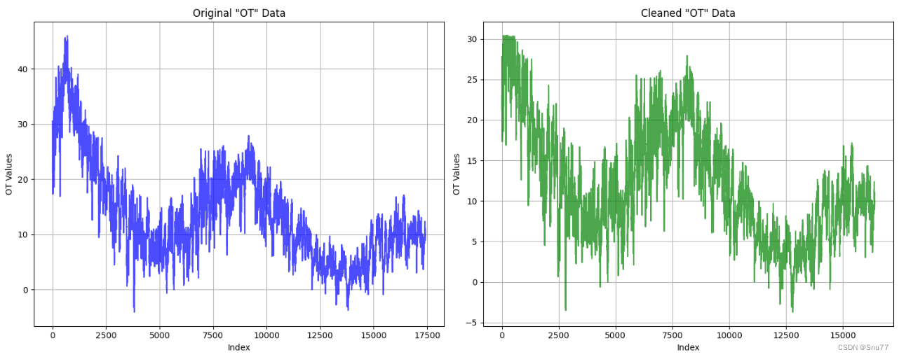
可以明显的看到当我们使用将异常值删除之后我们的数据范围从(40,-5)来到了(30,-5)数据范围变得更窄,起到了一定数据平缓的作用,让数据的波动性变小从而提高模型的预测精度(当然在实际中及其不推荐使用这种方法,因为这会破坏数据的周期性)。
4.2 替换法
4.2.1 平均值替换
平均值替换:用整个数据集的平均值替换异常值。
推荐指数:⭐⭐⭐
import pandas as pd
from scipy.stats import zscore
import matplotlib.pyplot as plt

# Load the data
file_path = 'ETTh1.csv'  # Replace with your file path
data = pd.read_csv(file_path)

# Calculate Z-Scores for the 'OT' column
data['OT_ZScore'] = zscore(data['OT'])

# Filter out rows where the Z-Score is greater than 2
outliers_removed = data[data['OT_ZScore'].abs() <= 2]

# Creating a figure with two subplots
fig, axes = plt.subplots(nrows=1, ncols=2, figsize=(15, 6))

# Plotting the original data in the first subplot
axes[0].plot(data['OT'], label='Original Data', color='blue', alpha=0.7)
axes[0].set_title('Original "OT" Data')
axes[0].set_xlabel('Index')
axes[0].set_ylabel('OT Values')
axes[0].grid(True)

# Plotting the cleaned data in the second subplot
axes[1].plot(outliers_removed['OT'].reset_index(drop=True), label='Mean Value Replacement', color='green', alpha=0.7)
axes[1].set_title('Cleaned "OT" Data')
axes[1].set_xlabel('Index')
axes[1].set_ylabel('OT Values')
axes[1].grid(True)

# Adjusting layout and displaying the plot
plt.tight_layout()
plt.show()

可以看到这种方法的效果和上面的删除差多,在实际使用中平均值使用替换可以算做一种保守的方法。
4.2.2 中位数替换
中位数替换:用中位数来替换异常值,尤其适用于数据不对称分布的情况。
推荐指数:⭐⭐⭐⭐
import pandas as pd
from scipy.stats import zscore
import matplotlib.pyplot as plt

# Load the data
file_path = 'ETTh1.csv'  # Replace with your file path
data = pd.read_csv(file_path)

# Calculate Z-Scores for the 'OT' column
data['OT_ZScore'] = zscore(data['OT'])

# Filter out rows where the Z-Score is greater than 2
outliers_removed = data[data['OT_ZScore'].abs() <= 2]

# Creating a figure with two subplots
fig, axes = plt.subplots(nrows=1, ncols=2, figsize=(15, 6))

# Plotting the original data in the first subplot
axes[0].plot(data['OT'], label='Original Data', color='blue', alpha=0.7)
axes[0].set_title('Original "OT" Data')
axes[0].set_xlabel('Index')
axes[0].set_ylabel('OT Values')
axes[0].grid(True)

# Plotting the cleaned data in the second subplot
axes[1].plot(outliers_removed['OT'].reset_index(drop=True), label='Median Value Replacement', color='green', alpha=0.7)
axes[1].set_title('Cleaned "OT" Data')
axes[1].set_xlabel('Index')
axes[1].set_ylabel('OT Values')
axes[1].grid(True)

# Adjusting layout and displaying the plot
plt.tight_layout()
plt.show()

大家由这两张图片可以看出替换法的效果都差不多。
4.2.3 众数替换
众数替换:对于分类数据,可以使用众数来替换异常值。
推荐指数:⭐⭐⭐⭐
import pandas as pd
from scipy.stats import zscore
import matplotlib.pyplot as plt

# Load the data
file_path = 'ETTh1.csv'  # Replace with your file path
data = pd.read_csv(file_path)

# Calculate Z-Scores for the 'OT' column
data['OT_ZScore'] = zscore(data['OT'])

# Filter out rows where the Z-Score is greater than 2
outliers_removed = data[data['OT_ZScore'].abs() <= 2]

# Creating a figure with two subplots
fig, axes = plt.subplots(nrows=1, ncols=2, figsize=(15, 6))

# Plotting the original data in the first subplot
axes[0].plot(data['OT'], label='Original Data', color='blue', alpha=0.7)
axes[0].set_title('Original "OT" Data')
axes[0].set_xlabel('Index')
axes[0].set_ylabel('OT Values')
axes[0].grid(True)

# Plotting the cleaned data in the second subplot
axes[1].plot(outliers_removed['OT'].reset_index(drop=True), label='Mode Value Replacement', color='green', alpha=0.7)
axes[1].set_title('Cleaned "OT" Data')
axes[1].set_xlabel('Index')
axes[1].set_ylabel('OT Values')
axes[1].grid(True)

# Adjusting layout and displaying the plot
plt.tight_layout()
plt.show()
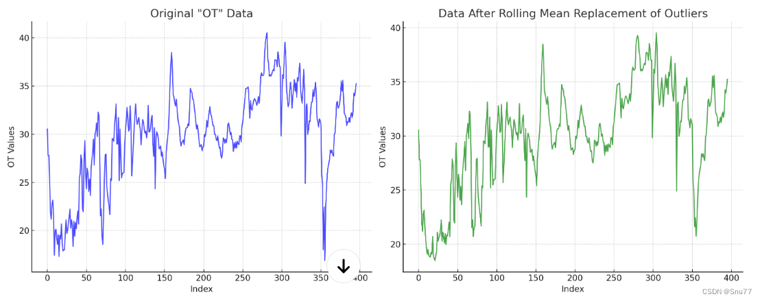
4.2.4 移动平滑替换
移动平滑替换:用异常值附近的平均值替换,需要设定一个窗口大小
推荐指数:⭐⭐⭐⭐⭐
import pandas as pd
import numpy as np
import matplotlib.pyplot as plt
from scipy.stats import zscore

# Load the data
file_path = 'your_file_path_here.csv'  # Replace with your file path
data = pd.read_csv(file_path)

# Calculate Z-Scores for the 'OT' column
data['OT_ZScore'] = zscore(data['OT'])

# Setting a default window size for rolling mean
window_size = 5

# Calculate the rolling mean
rolling_mean = data['OT'].rolling(window=window_size, center=True).mean()

# Replace outliers (Z-Score > 2) with the rolling mean
data['OT_RollingMean'] = data.apply(lambda row: rolling_mean[row.name] if abs(row['OT_ZScore']) > 2 else row['OT'], axis=1)

# Creating a figure with two subplots
fig, axes = plt.subplots(nrows=1, ncols=2, figsize=(15, 6))

# Plotting the original data in the first subplot
axes[0].plot(data['OT'], label='Original Data', color='blue', alpha=0.7)
axes[0].set_title('Original "OT" Data')
axes[0].set_xlabel('Index')
axes[0].set_ylabel('OT Values')
axes[0].grid(True)

# Plotting the data after replacing outliers with rolling mean in the second subplot
axes[1].plot(data['OT_RollingMean'], label='Data After Rolling Mean Replacement', color='green', alpha=0.7)
axes[1].set_title('Data After Rolling Mean Replacement of Outliers')
axes[1].set_xlabel('Index')
axes[1].set_ylabel('OT Values')
axes[1].grid(True)

# Adjusting layout and displaying the plot
plt.tight_layout()
plt.show()
4.3 变换法
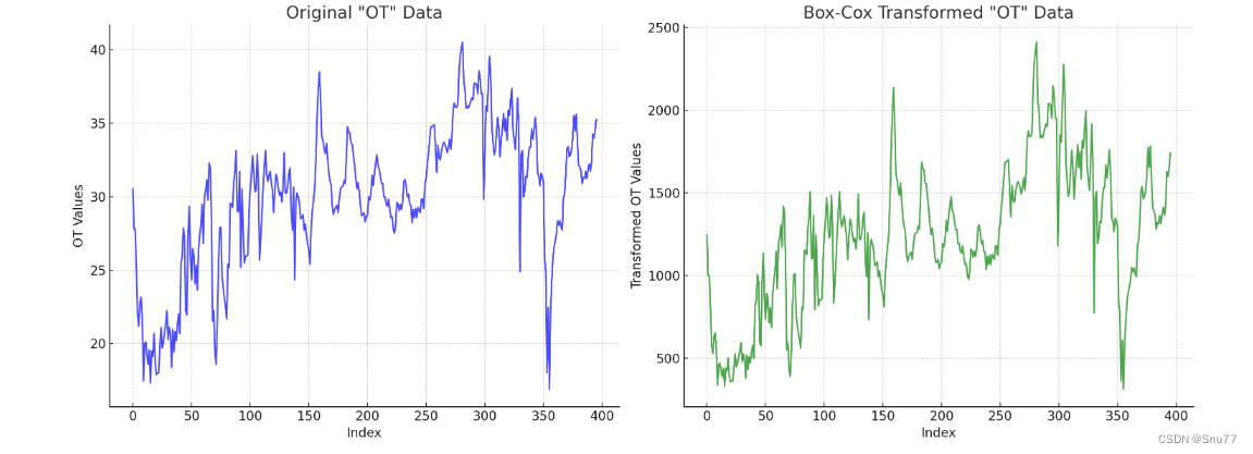
4.3.1 Box-Cox变化
Box-Cox变换:一种通用的转换方法,可以处理各种类型的偏态分布。
推荐指数:⭐⭐⭐
大家再用这种方法的时候需要注意数据中不能包含负值
import pandas as pd
from scipy.stats import zscore, boxcox
import matplotlib.pyplot as plt

# Load the data
file_path = 'ETTh1.csv'  # Replace with your file path
data = pd.read_csv(file_path)

# Calculate Z-Scores for the 'OT' column
data['OT_ZScore'] = zscore(data['OT'])

# Filter out rows where the Z-Score is greater than 2
outliers_removed = data[data['OT_ZScore'].abs() <= 2]

# Applying Box-Cox transformation
data['OT_BoxCox'], _ = boxcox(data['OT'])

# Creating a figure with two subplots
fig, axes = plt.subplots(nrows=1, ncols=2, figsize=(15, 6))

# Plotting the original data in the first subplot
axes[0].plot(data['OT'], label='Original Data', color='blue', alpha=0.7)
axes[0].set_title('Original "OT" Data')
axes[0].set_xlabel('Index')
axes[0].set_ylabel('OT Values')
axes[0].grid(True)

# Plotting the Box-Cox transformed data in the second subplot
axes[1].plot(data['OT_BoxCox'], label='Box-Cox Transformed Data', color='green', alpha=0.7)
axes[1].set_title('Box-Cox Transformed "OT" Data')
axes[1].set_xlabel('Index')
axes[1].set_ylabel('Transformed OT Values')
axes[1].grid(True)

# Adjusting layout and displaying the plot
plt.tight_layout()
plt.show()
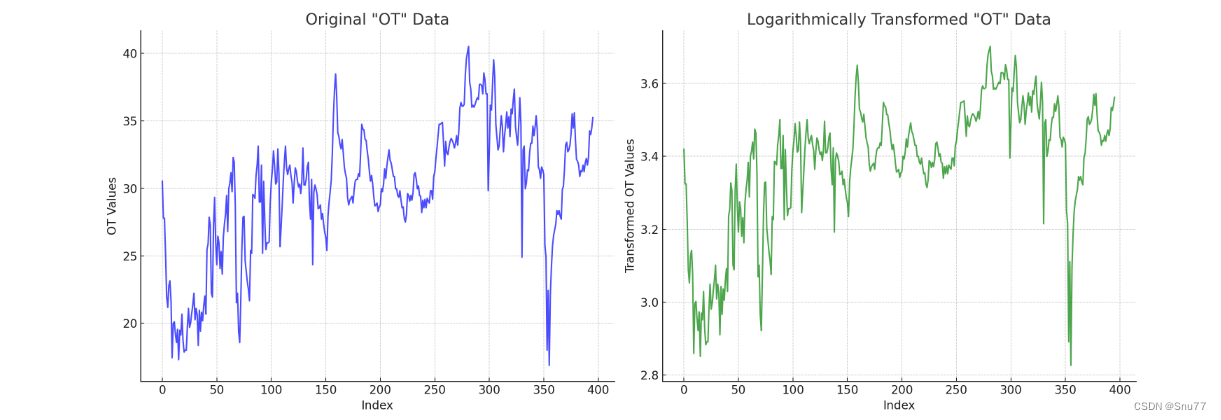
4.3.2 对数变化
对数变换:适用于右偏数据,可以减少数据的偏斜。
推荐指数:⭐
这个方法同理也不能输入负数,同时这个方法在我们输入到模型之后,输出结果之后还要将结果转换回来,实际是不推荐大家使用的。
import pandas as pd
import numpy as np
import matplotlib.pyplot as plt

# Load the data
file_path = 'ETTh1.csv'  # Replace with your file path
data = pd.read_csv(file_path)

# Replace values in 'OT' column that are less than 0 with the mean of the column
ot_mean = data['OT'].mean()
data['OT'] = data['OT'].apply(lambda x: ot_mean if x < 0 else x)

# Applying logarithmic transformation
data['OT_Log'] = np.log(data['OT'])

# Creating a figure with two subplots
fig, axes = plt.subplots(nrows=1, ncols=2, figsize=(15, 6))

# Plotting the original data in the first subplot
axes[0].plot(data['OT'], label='Original Data', color='blue', alpha=0.7)
axes[0].set_title('Original "OT" Data')
axes[0].set_xlabel('Index')
axes[0].set_ylabel('OT Values')
axes[0].grid(True)

# Plotting the logarithmically transformed data in the second subplot
axes[1].plot(data['OT_Log'], label='Logarithmically Transformed Data', color='green', alpha=0.7)
axes[1].set_title('Logarithmically Transformed "OT" Data')
axes[1].set_xlabel('Index')
axes[1].set_ylabel('Transformed OT Values')
axes[1].grid(True)

# Adjusting layout and displaying the plot
plt.tight_layout()
plt.show()
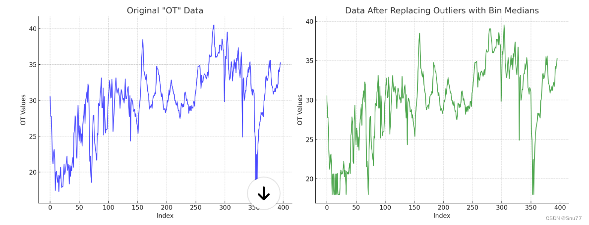
4.4 分箱法
分箱法:将数据分成几个区间(箱子),然后用箱子的边界值或中值来替换异常值。
推荐指数:⭐⭐⭐
import pandas as pd
import numpy as np
import matplotlib.pyplot as plt
from scipy.stats import zscore

# Load the data
file_path = 'your_file_path_here.csv'  # Replace with your file path
data = pd.read_csv(file_path)

# Calculate Z-Scores for the 'OT' column
data['OT_ZScore'] = zscore(data['OT'])

# Performing equal-width binning
num_bins = 10
data['OT_Binned'] = pd.cut(data['OT'], bins=num_bins)

# Calculating the median of each bin
binned_median = data.groupby('OT_Binned')['OT'].median()

# Replacing outliers with the median of the corresponding bin
data['OT_Replaced'] = data['OT'].copy()  # Creating a copy of the 'OT' column for replacements
for bin_interval, median_value in binned_median.items():
    # Find indices of outliers in this bin
    indices = data[(data['OT_Binned'] == bin_interval) & (data['OT_ZScore'].abs() > 2)].index
    # Replace these outliers with the median value of the bin
    data.loc[indices, 'OT_Replaced'] = median_value

# Creating a figure with two subplots
fig, axes = plt.subplots(nrows=1, ncols=2, figsize=(15, 6))

# Plotting the original data in the first subplot
axes[0].plot(data['OT'], label='Original Data', color='blue', alpha=0.7)
axes[0].set_title('Original "OT" Data')
axes[0].set_xlabel('Index')
axes[0].set_ylabel('OT Values')
axes[0].grid(True)

# Plotting the data after replacing outliers in the second subplot
axes[1].plot(data['OT_Replaced'], label='Data After Replacing Outliers', color='green', alpha=0.7)
axes[1].set_title('Data After Replacing Outliers with Bin Medians')
axes[1].set_xlabel('Index')
axes[1].set_ylabel('OT Values')
axes[1].grid(True)

# Adjusting layout and displaying the plot
plt.tight_layout()
plt.show()
4.5 使用机器学习模型
这种方法暂时不给大家介绍了,因为这就是时间序列预测,通过预测值来替换这个值,所以想用这种方法可以看我专栏里的其它内容。
推荐指数:⭐⭐
4.6 基于规则的方法
这种方法就是需要你有特定的知识,当我们用异常值检测方法检测出异常值之后去手动修改文件,其实这种是最合理的但是需要费时。
推荐指数:⭐⭐⭐⭐
五、全文总结
到此本文已经全部讲解完成了,希望能够帮助到大家,在这里也给大家推荐一些我其它的博客的时间序列实战案例讲解,其中有数据分析的讲解就是我前面提到的如何设置参数的分析博客,最后希望大家订阅我的专栏,本专栏均分文章均分98,并且免费阅读。
专栏回顾->时间序列预测专栏——包含上百种时间序列模型带你从入门到精通时间序列预测