【LSTM】北京pm2.5 天气预测--pytorch版本,有代码可以跑通-LSTM回归问题，工程落地一网打尽

文章目录

前言
1. 知识理解
- 1.1 核心理解
- 1.2 原理
- - 1.2.1 图解LSTM
  - 1.2.1 分词
  - 1.2.1 英语的词表示
  - 1.2.2 中文的词表示
  - 1.2.3 构建词表
2. 工程代码
- 2.1 数据预处理
- 2.2 数据集&模型构建
- 2.3 模型训练
- 2.4 保持模型&加载模型&预测

前言

LSTM 少分析原理，更强调工程落地，今年年初有两篇LSTM的回归文章，是keras实现的。
《【LSTM】LSTM预测股票价格–单因素、多步、输出单步回归特征 -keras 1》https://blog.csdn.net/weixin_40293999/article/details/128635150
《【LSTM】多因素单步骤预测-keras 2》http://t.csdnimg.cn/vRmMe

LSTM：做回归预测的几个应用。

1. 知识理解

1.1 核心理解

核心点:m个步长，n个因素，预测p个步长q个因素。
用前一天的日均温，预测当前天的日均温度—>1 步长 1 因素预测 1步长 1因素
用前一天的日均温、光照时长、风速、湿度预测当前天的日均温–>1 步长 4因素预测 1步长 1因素
用前一天的光照时长、风速、湿度预测当前天的日均温–>1 步长 3因素预测 1步长 1因素
用前7天的光照时长、风速、湿度预测后三天的日均温–> 7步长 3因素预测 3步长 1因素
用前7天的光照时长、风速、湿度预测后三天的日均温、光照时长、风速、湿度–> 7步长 3因素预测 3步长 4因素
通过以上的例子，相信你就能明白lstm做回归任务，能做什么。

关于其原理，自行搜索下其它人的讲解即可。本篇主要讲落地细节。

1.2 原理

1.2.1 图解LSTM

原理 ref: https://colah.github.io/posts/2015-08-Understanding-LSTMs/
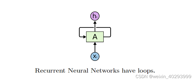
RNN:
在这里插入图片描述

LSTM:

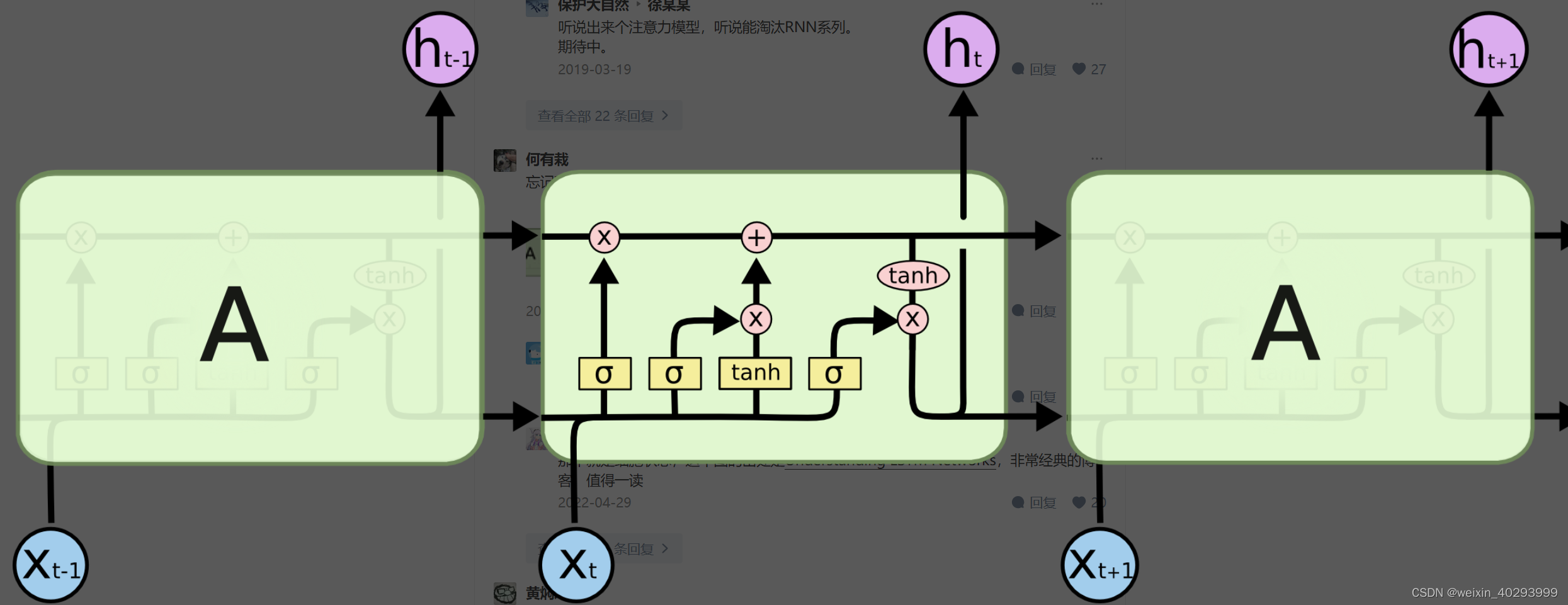
这张图挺好理解的：这个简洁来说就像个全加器一样，输出和进位都靠上一位的进位和本位的输入，挺好理解的

问题:特征 x1, x2,…xt 这t个x 对应的是什么？
就是一组特征向量，比如可以使7天的温度【一维向量 7】，也可以是7天的多维向量温度、湿度【二维向量 7X2】

1.2.1 分词

温度/湿度本身就是数字，但是若是影评数据呢？比如当幸福来敲门的台词：
You got a dream, you gotta protect it. Dont ever let somebody tell you, you can’t do something. Not even me. People can’t do something themselves, they wanna tell you,you can’t do it.
1）去标点 2）转成全小写 3）按 “ ”【空格】分词

s = "You got a dream, you gotta protect it. Dont ever let somebody tell you, you can't  do something. Not even me. People can't do something themselves, they wanna tell you,you can't do it."
import string
print("punctuation::",string.punctuation)
for c in string.punctuation:
    s = s.replace(c,' ').lower()
print("after deal with punctuation::",s)

punctuation:: !"#$%&'()*+,-./:;<=>?@[\]^_`{|}~
after deal with punctuation:: you got a dream  you gotta protect it  dont ever let somebody tell you  you can t  do something  not even me  people can t do something themselves  they wanna tell you you can t do it

np.unique(s.split())

array(['a', 'can', 'do', 'dont', 'dream', 'even', 'ever', 'got', 'gotta',
       'it', 'let', 'me', 'not', 'people', 'protect', 'somebody',
       'something', 't', 'tell', 'themselves', 'they', 'wanna', 'you'],
      dtype='<U10')

然后把这些词挨个变成映射【字典】，再用100维的张量表示每一个单词即可。

1.2.1 英语的词表示

这里说的特征就是数字类的，而不是文本类的比如影评、商品评价、外卖评价等等。
多啰嗦一句，其实一个英文影评（同步类比外卖、商品评价）的单词数量，就是 x1，x2，…xt, 对应的是t个单词。但是torch只能计算，只能存储float，int…等数字类型的tensor，你这个文本算个啥，所以需要将英语表示为【数字】特征，也就是词表示【word representation】，通常使用词嵌入【word embedding】的方式。每个单词可以表示为n维度，比如200，这个可以自定义，也可以用预训练的。

1.2.2 中文的词表示

1.2.1 说清楚了英文的词表示，那么中文呢，中文和英语其实极为相似，但是最大的不同是，英语很好分词，因为天然的空格存在，按空格分词【token】，再词表示就可以，中文没空咋给一句话【一段话】分词呢？用个插件jieba即可。
例子：

jieba.lcut("你说过两天来看我，转眼就是一年多！")
['你', '说', '过', '两天', '来看', '我', '，', '转眼', '就是', '一年', '多', '！']

1.2.3 构建词表

所以无论中英文，都需要构建词表，也就是分好词的所有词的list，比如所用影评分好词后的unique词是3W个，那么我们实际上就有一个len=3W的词表，
但通常还需要另外的两个词和。因为数据对齐的问题，比如我们就想让一条评论是200【多少的长度是自己定的】个单词。那多了，就截断了，少的就用填充。
另外，还需要一个注意点，就是从set【集合】的角度看，词表有3W个，但里面可能有只出现过1次的，他们可能是生僻词，或者拼写错误的，没啥具体含义。所以，做映射的时候，可能制取词频>=10的。那么没取到的，就被映射为unknow了。
然后，再用1.2的词表示。这样，一条评论。最终就是 200个单词，每个单词用100维的向量【数字】来表示。这样就和1.1的原理完全对上了。

2. 工程代码

2.1 数据预处理

在这里插入图片描述
pandas 读取数据，并完成预处理
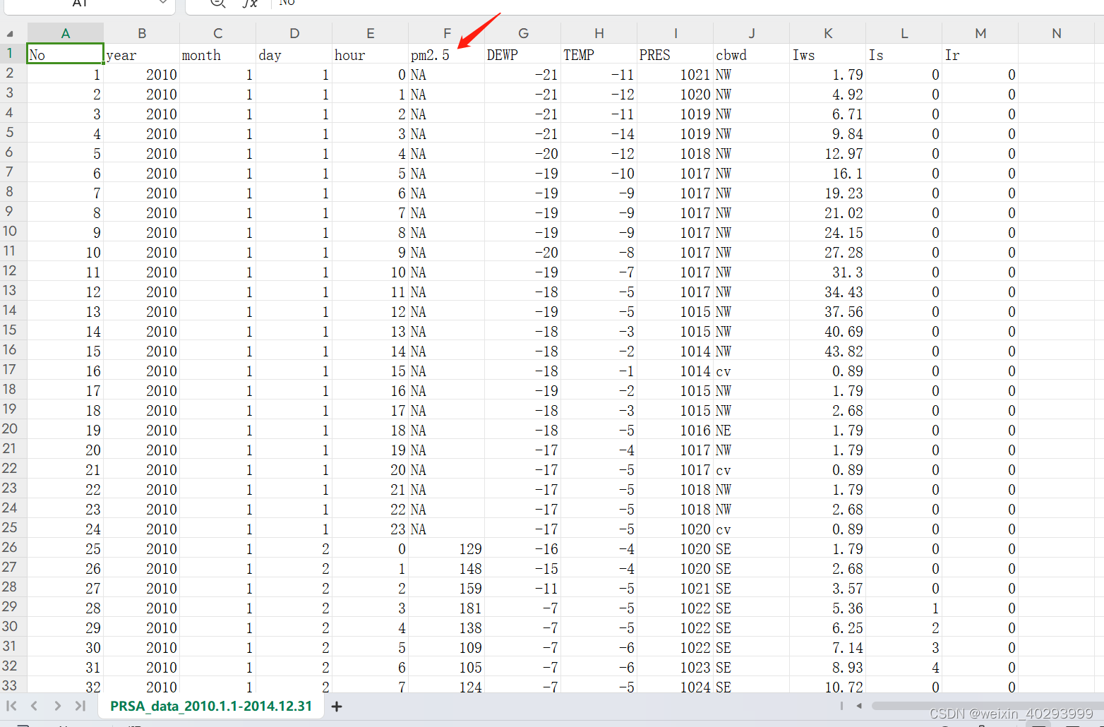
No year month day hour pm2.5 DEWP TEMP PRES cbwd Iws Is Ir
0 1 2010 1 1 0 NaN -21 -11.0 1021.0 NW 1.79 0 0
1 2 2010 1 1 1 NaN -21 -12.0 1020.0 NW 4.92 0 0
2 3 2010 1 1 2 NaN -21 -11.0 1019.0 NW 6.71 0 0
3 4 2010 1 1 3 NaN -21 -14.0 1019.0 NW 9.84 0 0
4 5 2010 1 1 4 NaN -20 -12.0 1018.0 NW 12.97 0 0

数据处理：把PM2.5 为null的数据都用相邻的数据填充，我们取2010年1月2日以后的数据。

data = data.iloc[24:].bfill()
print(data[0:5])

在这里插入图片描述
把年，月，日和小时合并为一列。

import datetime
data['time'] = data.apply(lambda x: datetime.datetime(year=x['year'],month =x['month'],day = x['day'],hour = x['hour']),axis = 1)

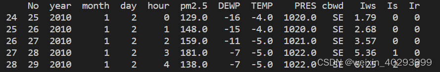
    No  year  month  day  hour  pm2.5  DEWP  TEMP    PRES cbwd   Iws  Is  Ir                time
24  25  2010      1    2     0  129.0   -16  -4.0  1020.0   SE  1.79   0   0 2010-01-02 00:00:00
25  26  2010      1    2     1  148.0   -15  -4.0  1020.0   SE  2.68   0   0 2010-01-02 01:00:00
26  27  2010      1    2     2  159.0   -11  -5.0  1021.0   SE  3.57   0   0 2010-01-02 02:00:00
27  28  2010      1    2     3  181.0    -7  -5.0  1022.0   SE  5.36   1   0 2010-01-02 03:00:00
28  29  2010      1    2     4  138.0    -7  -5.0  1022.0   SE  6.25   2   0 2010-01-02 04:00:

去掉年，月，日和小时，并且把时间列作为索引index

data.drop(columns=['No','year','month','day','hour'],inplace = True)
data = data.set_index('time')

                     pm2.5  DEWP  TEMP    PRES cbwd   Iws  Is  Ir
time
2010-01-02 00:00:00  129.0   -16  -4.0  1020.0   SE  1.79   0   0
2010-01-02 01:00:00  148.0   -15  -4.0  1020.0   SE  2.68   0   0
2010-01-02 02:00:00  159.0   -11  -5.0  1021.0   SE  3.57   0   0
2010-01-02 03:00:00  181.0    -7  -5.0  1022.0   SE  5.36   1   0
2010-01-02 04:00:00  138.0    -7  -5.0  1022.0   SE  6.25   2   0

One-hot 编码风向序列

data = data.join(pd.get_dummies(data.cbwd))
del data['cbwd']

                     pm2.5  DEWP  TEMP    PRES   Iws  Is  Ir     NE     NW    SE     cv
time
2010-01-02 00:00:00  129.0   -16  -4.0  1020.0  1.79   0   0  False  False  True  False
2010-01-02 01:00:00  148.0   -15  -4.0  1020.0  2.68   0   0  False  False  True  False
2010-01-02 02:00:00  159.0   -11  -5.0  1021.0  3.57   0   0  False  False  True  False
2010-01-02 03:00:00  181.0    -7  -5.0  1022.0  5.36   1   0  False  False  True  False
2010-01-02 04:00:00  138.0    -7  -5.0  1022.0  6.25   2   0  False  False  True  False

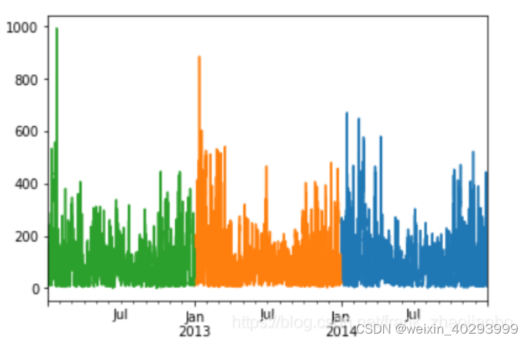
查看2012年到2014年的数据

data['pm2.5'][-365*24:].plot()
data['pm2.5'][-365*24*2:-365*24].plot()
data['pm2.5'][-365*24*3:-365*24*2].plot()

在这里插入图片描述
用前6天的数据预测第7天的大气PM2.5

sequence_length = 6*24
delay = 24
data_ = []
for i in range(len(data) - sequence_length - delay):
    data_.append(data.iloc[i: i + sequence_length + delay])
data_ = np.array([df.values for df in data_])
np.random.shuffle(data_)
x = data_[:, :-delay, :]
y = data_[:, -1, 0]

把数据的80%分成训练集合，20%分为测试集合。

split_boundary = int(data_.shape[0] * 0.8)
train_x = x[: split_boundary]
test_x = x[split_boundary:]

train_y = y[: split_boundary]
test_y = y[split_boundary:]

对数据标准化

mean = train_x.mean(axis=0) #均值
std = train_x.std(axis=0) #标准差
train_x = (train_x - mean)/std
test_x = (test_x - mean)/std

2.2 数据集&模型构建


class Mydataset(torch.utils.data.Dataset):
    def __init__(self, features, labels):
        self.features = features
        self.labels = labels
        
    def __getitem__(self, index):
        feature = self.features[index]
        label = self.labels[index]
        return feature, label

    def __len__(self):
        return len(self.features)
train_ds = Mydataset(train_x, train_y)
test_ds = Mydataset(test_x, test_y)
BTACH_SIZE = 128
train_dl = torch.utils.data.DataLoader(
                                       train_ds,
                                       batch_size=BTACH_SIZE,
                                       shuffle=True
)
test_dl = torch.utils.data.DataLoader(
                                       test_ds,
                                       batch_size=BTACH_SIZE
)

构建模型

hidden_size = 64
class Net(nn.Module):
    def __init__(self, hidden_size):
        super(Net, self).__init__()
        self.rnn = nn.LSTM(train_x.shape[-1], 
                           hidden_size, 
                           batch_first=True)
        self.fc1 = nn.Linear(hidden_size, 128)
        self.fc2 = nn.Linear(128, 1)

    def forward(self, inputs):
        _, s_o = self.rnn(inputs)
        s_o = s_o[-1]
        x = F.dropout(F.relu(self.fc1(s_o)))
        x = self.fc2(x)
        return torch.squeeze(x)
model = Net(hidden_size)
if torch.cuda.is_available():
    model.to('cuda')

构建损失和优化函数


loss_fn = nn.MSELoss()
optimizer = torch.optim.Adam(model.parameters(), lr=0.001)

2.3 模型训练

训练过程

def fit(epoch, model, trainloader, testloader):
    total = 0
    running_loss = 0
    
    model.train()
    for x, y in trainloader:
        if torch.cuda.is_available():
            x, y = x.to('cuda'), y.to('cuda')
        y_pred = model(x)
        loss = loss_fn(y_pred, y)
        optimizer.zero_grad()
        loss.backward()
        optimizer.step()
        with torch.no_grad():
            total += y.size(0)
            running_loss += loss.item()
#    exp_lr_scheduler.step()
    epoch_loss = running_loss / len(trainloader.dataset)
        
        
    test_total = 0
    test_running_loss = 0 
    
    model.eval()
    with torch.no_grad():
        for x, y in testloader:
            if torch.cuda.is_available():
                x, y = x.to('cuda'), y.to('cuda')
            y_pred = model(x)
            loss = loss_fn(y_pred, y)
            test_total += y.size(0)
            test_running_loss += loss.item()
    
    epoch_test_loss = test_running_loss / len(testloader.dataset)
    
        
    print('epoch: ', epoch, 
          'loss： ', round(epoch_loss, 3),
          'test_loss： ', round(epoch_test_loss, 3),
             )
        
    return epoch_loss, epoch_test_loss

epochs = 100
train_loss = []
test_loss = []

for epoch in range(epochs):
    epoch_loss, epoch_test_loss = fit(epoch,
                                      model,
                                      train_dl,
                                      test_dl)
    train_loss.append(epoch_loss)
    test_loss.append(epoch_test_loss)

训练过程loss


epoch:  0 loss：  23.613 test_loss：  25.115
epoch:  1 loss：  23.081 test_loss：  24.546
epoch:  2 loss：  22.261 test_loss：  23.605
epoch:  3 loss：  21.603 test_loss：  23.745
epoch:  4 loss：  21.623 test_loss：  24.013
epoch:  5 loss：  21.449 test_loss：  24.356
epoch:  6 loss：  21.052 test_loss：  22.461
epoch:  7 loss：  21.267 test_loss：  24.883
epoch:  8 loss：  21.083 test_loss：  21.641
epoch:  9 loss：  20.027 test_loss：  24.942
epoch:  10 loss：  19.944 test_loss：  20.995
epoch:  11 loss：  20.05 test_loss：  23.553
epoch:  12 loss：  30.013 test_loss：  29.03
epoch:  13 loss：  23.522 test_loss：  22.274
epoch:  14 loss：  20.181 test_loss：  21.099
epoch:  15 loss：  19.553 test_loss：  20.401
epoch:  16 loss：  18.925 test_loss：  21.033
epoch:  17 loss：  18.798 test_loss：  19.627
epoch:  18 loss：  19.772 test_loss：  20.952
epoch:  19 loss：  19.922 test_loss：  20.91
epoch:  20 loss：  19.068 test_loss：  20.825
epoch:  21 loss：  18.103 test_loss：  19.203
epoch:  22 loss：  19.176 test_loss：  20.891
epoch:  23 loss：  17.713 test_loss：  19.167
epoch:  24 loss：  17.063 test_loss：  18.672
epoch:  25 loss：  19.715 test_loss：  23.334
epoch:  26 loss：  21.586 test_loss：  20.307
epoch:  27 loss：  18.127 test_loss：  19.236
epoch:  28 loss：  16.943 test_loss：  18.996
epoch:  29 loss：  17.403 test_loss：  19.15
epoch:  30 loss：  16.35 test_loss：  18.142
epoch:  31 loss：  16.166 test_loss：  18.056
epoch:  32 loss：  16.363 test_loss：  20.465
epoch:  33 loss：  16.122 test_loss：  17.937
epoch:  34 loss：  15.48 test_loss：  17.128
epoch:  35 loss：  17.159 test_loss：  19.565
epoch:  36 loss：  18.402 test_loss：  22.737
epoch:  37 loss：  17.671 test_loss：  19.016
epoch:  38 loss：  16.368 test_loss：  17.944
epoch:  39 loss：  15.901 test_loss：  18.256
epoch:  40 loss：  15.695 test_loss：  18.299
epoch:  41 loss：  15.447 test_loss：  16.485
epoch:  42 loss：  14.995 test_loss：  16.351
epoch:  43 loss：  14.906 test_loss：  17.371
epoch:  44 loss：  14.784 test_loss：  16.312
epoch:  45 loss：  15.204 test_loss：  17.165
epoch:  46 loss：  15.076 test_loss：  16.702
epoch:  47 loss：  14.528 test_loss：  15.929
epoch:  48 loss：  14.185 test_loss：  31.667
epoch:  49 loss：  22.848 test_loss：  20.964

2.4 保持模型&加载模型&预测

# 模型参数保存
torch.save(model.state_dict(), 'model_param.pt')
# 模型参数加载
model = Net(...)
model.load_state_dict(torch.load('model_param.pt'))

data_test = data[-24*6:]
data_test = (data_test - mean)/std
data_test = data_test.to_numpy()
data_test = np.expand_dims(data_test,0)
pm = model(torch.from_numpy(data_test).float().cuda())