雷达检测及MATLAB仿真

文章目录

前言
一、雷达检测
二、Matlab 仿真
- 1、高斯和瑞利概率密度函数
- - ①、MATLAB 源码
  - ②、仿真
- 2、归一化门限相对虚警概率的曲线
- - ①、MATLAB 源码
  - ②、仿真
- 3、检测概率相对于单个脉冲 SNR 的关系曲线
- - ①、MATLAB 源码
  - ②、仿真
- 4、改善因子和积累损失相对于非相干积累脉冲数的关系曲线
- - ①、改善因子相对于非相干积累脉冲数的关系曲线
  - - 1）MATLAB 源码
    - 2）仿真
  - ②、积累损失相对于非相干积累脉冲数的关系曲线
  - - 1）MATLAB 源码
    - 2）仿真
- 5、起伏目标检测概率
- - ①、Swerling V 型目标的检测
  - - 1）MATLAB 源码
    - 2）仿真
  - ②、Swerling Ⅰ 型目标的检测
  - - 1）MATLAB 源码
    - 2）仿真
    - 3）MATLAB 源码
    - 4）仿真
  - ③、Swerling Ⅱ 型目标的检测
  - - 1）MATLAB 源码
    - 2）仿真
  - ④、Swerling Ⅲ 型目标的检测
  - - 1）MATLAB 源码
    - 2）仿真
  - ⑤、Swerling Ⅳ 型目标的检测
  - - 1）MATLAB 源码
    - 2）仿真
三、资源自取

前言

本文对雷达检测的内容以思维导图的形式呈现，有关仿真部分进行了讲解实现。

一、雷达检测

思维导图如下图所示，如有需求请到文章末尾端自取。
在这里插入图片描述

二、Matlab 仿真

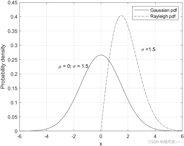
1、高斯和瑞利概率密度函数

瑞利概率密度函数： $f(x)=\frac{x}{\sigma^2}e^{-\frac{x^2}{2\sigma^2}}$

高斯概率密度函数： $\approx \frac{1}{\sqrt{2\pi\sigma^2}}e^{-\frac{(x-\mu)^2}{2\sigma^2}}$

$x$ 是变量， $\mu$ 是均值， $\sigma$ 是方差

①、MATLAB 源码

clear all
close all
xg = linspace(-6,6,1500); % randowm variable between -4 and 4
xr = linspace(0,6,1500); % randowm variable between 0 and 8
mu = 0; % zero mean Gaussain pdf mean
sigma = 1.5; % standard deviation (sqrt(variance) 
ynorm = normpdf(xg,mu,sigma); % use MATLAB funtion normpdf
yray = raylpdf(xr,sigma); % use MATLAB function raylpdf
plot(xg,ynorm,'k',xr,yray,'k-.');
grid
legend('Gaussian pdf','Rayleigh pdf')
xlabel('x')
ylabel('Probability density')
gtext('\mu = 0; \sigma = 1.5')
gtext('\sigma =1.5')

②、仿真

请添加图片描述

高斯和瑞利概率密度

2、归一化门限相对虚警概率的曲线

虚警概率： $P_{fa}=e^{\frac{-V_T^2}{2\psi^2}}$

门限电压： $V_T=\sqrt{2\psi^2ln(\frac{1}{P_{fa}})}$

注： $V_T$ 为门限电压， $\psi^2$ 为方差

①、MATLAB 源码

close all
clear all
logpfa = linspace(.01,250,1000);
var = 10.^(logpfa ./ 10.0);
vtnorm =  sqrt( log (var));
semilogx(logpfa, vtnorm,'k')
grid

②、仿真

横坐标为 $log(1/P_{fa})$
纵坐标为 $\frac{V_T}{\sqrt{2\psi^2}}$
请添加图片描述

归一化检测门限对虚警概率

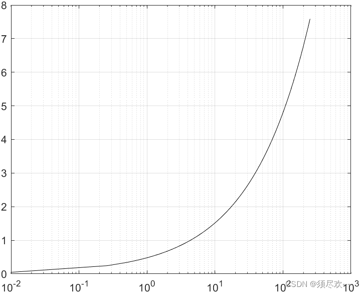
从图中可以明显看出， $P_{fa}$ 对门限值的小变化非常敏感

3、检测概率相对于单个脉冲 SNR 的关系曲线

检测概率 $P_D$ ：
在这里插入图片描述
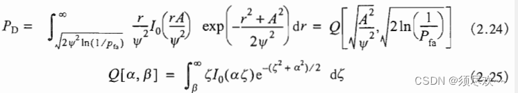
$Q$ 称为 $M a rc u m Q$ 函数。

①、MATLAB 源码

marcumsq.m

function PD = marcumsq (a,b)
% This function uses Parl's method to compute PD
max_test_value = 5000.; 
if (a < b)
   alphan0 = 1.0;
   dn = a / b;
else
   alphan0 = 0.;
   dn = b / a;
end
alphan_1 = 0.;
betan0 = 0.5;
betan_1 = 0.;
D1 = dn;
n = 0;
ratio = 2.0 / (a * b);
r1 = 0.0;
betan = 0.0;
alphan = 0.0;
while betan < 1000.,
   n = n + 1;
   alphan = dn + ratio * n * alphan0 + alphan;
   betan = 1.0 + ratio * n * betan0 + betan;
   alphan_1 = alphan0;
   alphan0 = alphan;
   betan_1 = betan0;
   betan0 = betan;
   dn = dn * D1;
end
PD = (alphan0 / (2.0 * betan0)) * exp( -(a-b)^2 / 2.0);
if ( a >= b)
   PD = 1.0 - PD;
end
return

prob_snr1.m

% This program is used to produce Fig. 2.4
close all
clear all
for nfa = 2:2:12
   b = sqrt(-2.0 * log(10^(-nfa)));
   index = 0;
   hold on
   for snr = 0:.1:18
      index = index +1;
      a = sqrt(2.0 * 10^(.1*snr));
      pro(index) = marcumsq(a,b);
   end
   x = 0:.1:18;
   set(gca,'ytick',[.1 .2 .3 .4 .5 .6  .7 .75 .8 .85 .9 ...
         .95 .9999])
   set(gca,'xtick',[1 2 3 4 5 6 7 8 9 10 11 12 13 14 15 16 17 18])

   loglog(x, pro,'k');
end
hold off
xlabel ('Single pulse SNR - dB')
ylabel ('Probability of detection')
grid

②、仿真

检测概率相对于单个脉冲 $SNR$ 的关系曲线对于 $P_{fa}$ 的个数值:

请添加图片描述
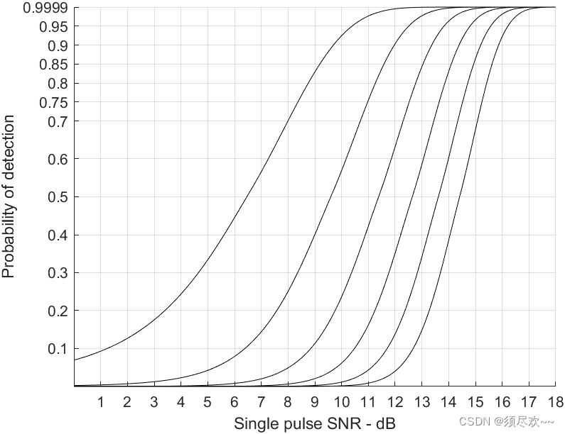
6 条曲线的 $P_{fa}$ 从左到右依次是 $10^{-2}，10^{-4}，10^{-6}，10^{-8}，10^{-10}，10^{-12}$ ，可以看到随着 SNR 信噪比的增加，检测概率逐渐增大，此外，虚警概率越小，随着信噪比的增加，检测概率增加的越快。

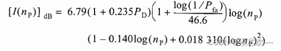
4、改善因子和积累损失相对于非相干积累脉冲数的关系曲线

$I(n_p)$ 称为积累改善因子

在这里插入图片描述

①、改善因子相对于非相干积累脉冲数的关系曲线

1）MATLAB 源码

improv_fac.m

function impr_of_np = improv_fac (np, pfa, pd)
% This function computes the non-coherent integration improvment
% factor using the empirical formula defind in Eq. (2.48)
fact1 = 1.0 + log10( 1.0 / pfa) / 46.6;
fact2 = 6.79 * (1.0 + 0.253 * pd);
fact3 = 1.0 - 0.14 * log10(np) + 0.0183 * (log10(np))^2;
impr_of_np = fact1 * fact2 * fact3 * log10(np);
return

fig2_6a.m

% This program is used to produce Fig. 2.6a
% It uses the function "improv_fac"
clear all
close all
pfa1 = 1.0e-2;
pfa2 = 1.0e-6;
pfa3 = 1.0e-10;
pfa4 = 1.0e-13;
pd1 = .5;
pd2 = .8;
pd3 = .95;
pd4 = .999;
index = 0;
for np = 1:1:1000
   index = index + 1;
   I1(index) = improv_fac (np, pfa1, pd1);
   I2(index) = improv_fac (np, pfa2, pd2);
   I3(index) = improv_fac (np, pfa3, pd3);
   I4(index) = improv_fac (np, pfa4, pd4);
end
np = 1:1:1000;
semilogx (np, I1, 'k', np, I2, 'k--', np, I3, 'k-.', np, I4, 'k:')
%set (gca,'xtick',[1 2 3 4 5 6 7 8  10 20 30 100]);
xlabel ('Number of pulses');
ylabel ('Improvement factor in dB')
legend ('pd=.5, nfa=e+2','pd=.8, nfa=e+6','pd=.95, nfa=e+10','pd=.999, nfa=e+13');
grid

2）仿真

请添加图片描述

改善因子相对于非相干积累脉冲数的关系曲线

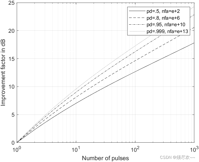
可以看到随着非相干积累脉冲数的增多，改善因子逐渐增大；在同一脉冲数的情况下，随着检测概率和虚警概率的增大，则改善因子也会逐渐增大

②、积累损失相对于非相干积累脉冲数的关系曲线

1）MATLAB 源码

% This program is used to produce Fig. 2.6b
% It uses the function "improv_fac". 
clear all
close all
pfa1 = 1.0e-12;
pfa2 = 1.0e-12;
pfa3 = 1.0e-12;
pfa4 = 1.0e-12;
pd1 = .5;
pd2 = .8;
pd3 = .95;
pd4 = .99;
index = 0;
for np = 1:1:1000
    index = index+1;
    I1 = improv_fac (np, pfa1, pd1);
    i1 = 10.^(0.1*I1);
    L1(index) = -1*10*log10(i1 ./ np);
    I2 = improv_fac (np, pfa2, pd2);
    i2 = 10.^(0.1*I2);
    L2(index) = -1*10*log10(i2 ./ np);
    I3 = improv_fac (np, pfa3, pd3);
    i3 = 10.^(0.1*I3);
    L3(index) = -1*10*log10(i3 ./ np);
    I4 = improv_fac (np, pfa4, pd4);
    i4 = 10.^(0.1*I4);
    L4 (index) = -1*10*log10(i4 ./ np);
end
np = 1:1:1000;
semilogx (np, L1, 'k', np, L2, 'k--', np, L3, 'k-.', np, L4, 'k:')
axis tight
xlabel ('Number of pulses');
ylabel ('Integration loss - dB')
legend ('pd=.5, nfa=e+12','pd=.8, nfa=e+12','pd=.95, nfa=e+12','pd=.99, nfa=e+12');
grid

2）仿真

请添加图片描述

积累损失相对于非相干积累脉冲数的关系曲线

可以看到随着非相干积累脉冲数的增多，积累损失逐渐增大；在同一脉冲数的情况下，随着检测概率的增大，则积累损失会逐渐减小

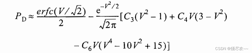
5、起伏目标检测概率

①、Swerling V 型目标的检测

检测概率 $P_D$ ：
在这里插入图片描述

$n_p=1,10$ 时检测概率相对于 SNR 的曲线

1）MATLAB 源码

pd_swerling5.m

function pd = pd_swerling5 (input1, indicator, np, snrbar)
% This function is used to calculate the probability of detection
% for Swerling 5 or 0 targets for np>1.
if(np == 1)
   'Stop, np must be greater than 1'
   return
end
format long
snrbar = 10.0.^(snrbar./10.);
eps = 0.00000001;
delmax = .00001;
delta =10000.;
% Calculate the threshold Vt
if (indicator ~=1)
   nfa = input1;
   pfa =  np * log(2) / nfa;
else
   pfa = input1;
   nfa = np * log(2) / pfa;
end
sqrtpfa = sqrt(-log10(pfa));
sqrtnp = sqrt(np); 
vt0 = np - sqrtnp + 2.3 * sqrtpfa * (sqrtpfa + sqrtnp - 1.0);
vt = vt0;
while (abs(delta) >= vt0)
   igf = incomplete_gamma(vt0,np);
   num = 0.5^(np/nfa) - igf;
   temp = (np-1) * log(vt0+eps) - vt0 - factor(np-1);
   deno = exp(temp);
   vt = vt0 + (num / (deno+eps));
   delta = abs(vt - vt0) * 10000.0; 
   vt0 = vt;
end
% Calculate the Gram-Chrlier coeffcients
temp1 = 2.0 .* snrbar + 1.0;
omegabar = sqrt(np .* temp1);
c3 = -(snrbar + 1.0 / 3.0) ./ (sqrt(np) .* temp1.^1.5);
c4 = (snrbar + 0.25) ./ (np .* temp1.^2.);
c6 = c3 .* c3 ./2.0;
V = (vt - np .* (1.0 + snrbar)) ./ omegabar;
Vsqr = V .*V;
val1 = exp(-Vsqr ./ 2.0) ./ sqrt( 2.0 * pi);
val2 = c3 .* (V.^2 -1.0) + c4 .* V .* (3.0 - V.^2) -...
   c6 .* V .* (V.^4 - 10. .* V.^2 + 15.0);
q = 0.5 .* erfc (V./sqrt(2.0));
pd =  q - val1 .* val2;

在这里插入图片描述

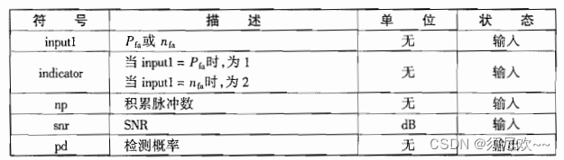
fig2_9.m

close all
clear all
pfa = 1e-9;
nfa = log(2) / pfa;
b = sqrt(-2.0 * log(pfa));
index = 0;
for snr = 0:.1:20
   index = index +1;
   a = sqrt(2.0 * 10^(.1*snr));
   pro(index) = marcumsq(a,b);
   prob205(index) =  pd_swerling5 (pfa, 1, 10, snr);
end
x = 0:.1:20;
plot(x, pro,'k',x,prob205,'k:');
axis([0 20 0 1])
xlabel ('SNR - dB')
ylabel ('Probability of detection')
legend('np = 1','np = 10')
grid

2）仿真

$n_p=1,10$ 时检测概率相对于 SNR 的曲线
请添加图片描述
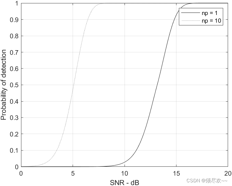
注意到为了获得同样的检概率，10 个脉冲非相干积累比单个脉冲需要更少的 SNR。

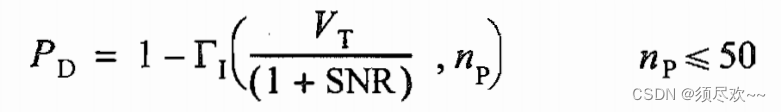
②、Swerling Ⅰ 型目标的检测

检测概率 $P_D$ ：
在这里插入图片描述

1）MATLAB 源码

pd_swerling2.m

function pd = pd_swerling2 (nfa, np, snrbar)
% This function is used to calculate the probability of detection
% for Swerling 2 targets.
format long
snrbar = 10.0^(snrbar/10.);
eps = 0.00000001;
delmax = .00001;
delta =10000.;
% Calculate the threshold Vt
pfa =  np * log(2) / nfa;
sqrtpfa = sqrt(-log10(pfa));
sqrtnp = sqrt(np); 
vt0 = np - sqrtnp + 2.3 * sqrtpfa * (sqrtpfa + sqrtnp - 1.0);
vt = vt0;
while (abs(delta) >= vt0)
   igf = incomplete_gamma(vt0,np);
   num = 0.5^(np/nfa) - igf;
   temp = (np-1) * log(vt0+eps) - vt0 - factor(np-1);
   deno = exp(temp);
   vt = vt0 + (num / (deno+eps));
   delta = abs(vt - vt0) * 10000.0; 
   vt0 = vt;
end
if (np <= 50)
   temp = vt / (1.0 + snrbar);
   pd = 1.0 - incomplete_gamma(temp,np);
   return
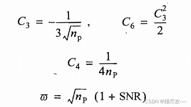
else
   temp1 = snrbar + 1.0;
   omegabar = sqrt(np) * temp1;
   c3 = -1.0 / sqrt(9.0 * np);
   c4 = 0.25 / np;
   c6 = c3 * c3 /2.0;
   V = (vt - np * temp1) / omegabar;
   Vsqr = V *V;
   val1 = exp(-Vsqr / 2.0) / sqrt( 2.0 * pi);
   val2 = c3 * (V^2 -1.0) + c4 * V * (3.0 - V^2) - ... 
      c6 * V * (V^4 - 10. * V^2 + 15.0);
   q = 0.5 * erfc (V/sqrt(2.0));
   pd =  q - val1 * val2;
end

在这里插入图片描述
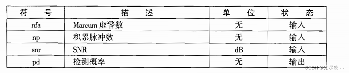
fig2_10.m

clear all
pfa = 1e-9;
nfa = log(2) / pfa;
b = sqrt(-2.0 * log(pfa));
index = 0;
for snr = 0:.01:22
   index = index +1;
   a = sqrt(2.0 * 10^(.1*snr));
   pro(index) = marcumsq(a,b);
   prob(index) =  pd_swerling2 (nfa, 1, snr);
end
x = 0:.01:22;
%figure(10)
plot(x, pro,'k',x,prob,'k:');
axis([2 22 0 1])
xlabel ('SNR - dB')
ylabel ('Probability of detection')
legend('Swerling V','Swerling I')
grid

2）仿真

检测概率相对于 SNR，单个脉冲， $P_{fa}=10^{-9}$ ：
请添加图片描述
可以看出为了获得与无起伏情况相同的 $P_D$ ，在有起伏时，需要更高的 SNR。

3）MATLAB 源码

pd_swerling1.m

function pd = pd_swerling1 (nfa, np, snrbar)
% This function is used to calculate the probability of detection
% for Swerling 1 targets.
format long
snrbar = 10.0^(snrbar/10.);
eps = 0.00000001;
delmax = .00001;
delta =10000.;
% Calculate the threshold Vt
pfa =  np * log(2) / nfa;
sqrtpfa = sqrt(-log10(pfa));
sqrtnp = sqrt(np); 
vt0 = np - sqrtnp + 2.3 * sqrtpfa * (sqrtpfa + sqrtnp - 1.0);
vt = vt0;
while (abs(delta) >= vt0)
   igf = incomplete_gamma(vt0,np);
   num = 0.5^(np/nfa) - igf;
   temp = (np-1) * log(vt0+eps) - vt0 - factor(np-1);
   deno = exp(temp);
   vt = vt0 + (num / (deno+eps));
   delta = abs(vt - vt0) * 10000.0; 
   vt0 = vt;
end
if (np == 1)
   temp = -vt / (1.0 + snrbar);
   pd = exp(temp);
   return
end
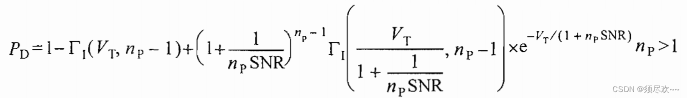
   temp1 = 1.0 + np * snrbar;
   temp2 = 1.0 / (np *snrbar);
   temp = 1.0 + temp2;
   val1 = temp^(np-1.);
   igf1 = incomplete_gamma(vt,np-1);
   igf2 = incomplete_gamma(vt/temp,np-1);
   pd = 1.0 - igf1 + val1 * igf2 * exp(-vt/temp1);

fig2_11ab.m

clear all
pfa = 1e-11;
nfa = log(2) / pfa;
index = 0;
for snr = -10:.5:30
   index = index +1;
   prob1(index) =  pd_swerling1 (nfa, 1, snr);
   prob10(index) =  pd_swerling1 (nfa, 10, snr);
   prob50(index) =  pd_swerling1 (nfa, 50, snr);
   prob100(index) =  pd_swerling1 (nfa, 100, snr);
end
x = -10:.5:30;
plot(x, prob1,'k',x,prob10,'k:',x,prob50,'k--', ...
   x, prob100,'k-.');
axis([-10 30 0 1])
xlabel ('SNR - dB')
ylabel ('Probability of detection')
legend('np = 1','np = 10','np = 50','np = 100')
grid

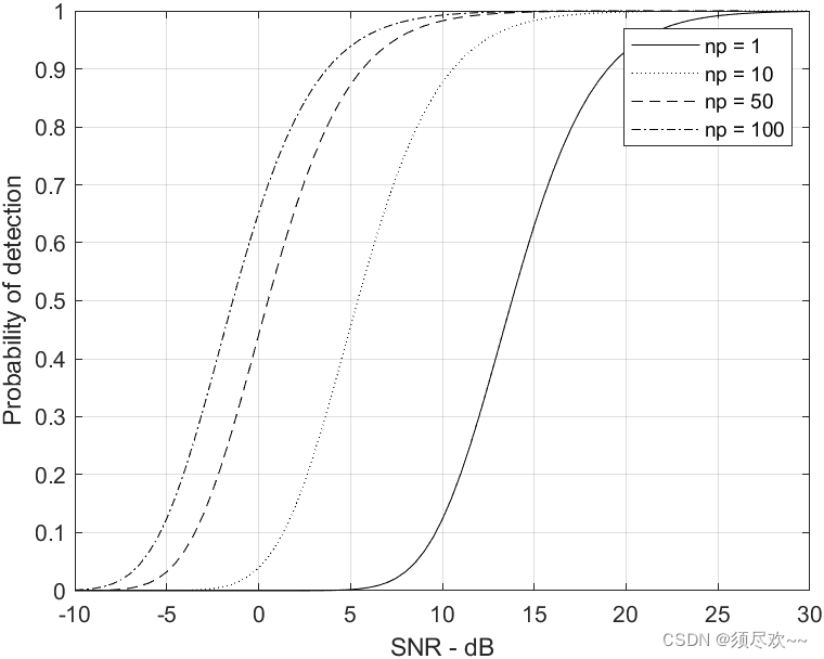
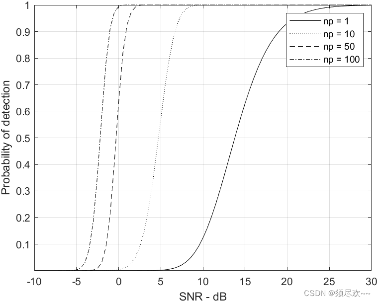
4）仿真

检测概率相对于 SNR，Swerling Ⅰ， $P_{fa}=10^{-8}$
请添加图片描述
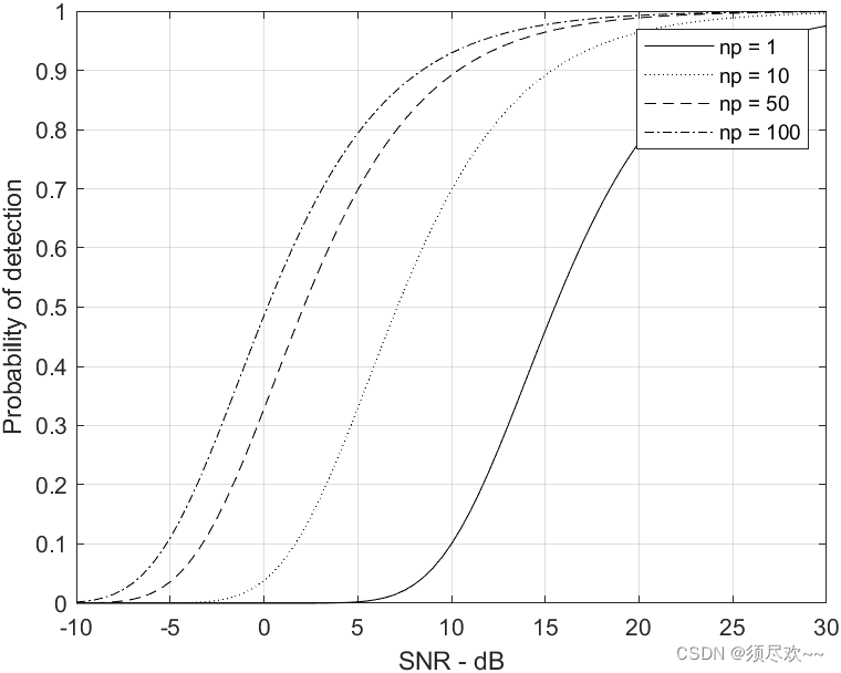
上图显示了 $n_p=1，10，50，100$ 时，检测概率相对于 SNR 的曲线，其中 $P_{fa}=10^{-8}$ ，可以看到 $n_p$ 越大，那么达到同一检测概率的 SNR 越小。

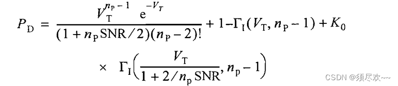
③、Swerling Ⅱ 型目标的检测

检测概率 $P_D$ ：
在这里插入图片描述
当 $n_p > 50$ 时：

此时：

1）MATLAB 源码

fig2_12.m

clear all
pfa = 1e-10;
nfa = log(2) / pfa;
index = 0;
for snr = -10:.5:30
   index = index +1;
   prob1(index) =  pd_swerling2 (nfa, 1, snr);
   prob10(index) =  pd_swerling2 (nfa, 10, snr);
   prob50(index) =  pd_swerling2 (nfa, 50, snr);
   prob100(index) =  pd_swerling2 (nfa, 100, snr);
end
x = -10:.5:30;
plot(x, prob1,'k',x,prob10,'k:',x,prob50,'k--', ...
   x, prob100,'k-.');
axis([-10 30 0 1])
xlabel ('SNR - dB')
ylabel ('Probability of detection')
legend('np = 1','np = 10','np = 50','np = 100')
grid

2）仿真

检测概率相对于 SNR，Swerling Ⅱ， $P_{fa}=10^{-10}$
请添加图片描述
上图显示了当 $n_p=1，10，50，100$ 时，检测概率作为 SNR 函数的曲线，其中 $P_{fa}=10^{-10}$

④、Swerling Ⅲ 型目标的检测

检测概率 $P_D$ ：
$n_p=1，2$ 时：
在这里插入图片描述
$n_p>2$ 时：

1）MATLAB 源码

pd_swerling3.m

function pd = pd_swerling3 (nfa, np, snrbar)
% This function is used to calculate the probability of detection
% for Swerling 2 targets.
format long
snrbar = 10.0^(snrbar/10.);
eps = 0.00000001;
delmax = .00001;
delta =10000.;
% Calculate the threshold Vt
pfa =  np * log(2) / nfa;
sqrtpfa = sqrt(-log10(pfa));
sqrtnp = sqrt(np); 
vt0 = np - sqrtnp + 2.3 * sqrtpfa * (sqrtpfa + sqrtnp - 1.0);
vt = vt0;
while (abs(delta) >= vt0)
   igf = incomplete_gamma(vt0,np);
   num = 0.5^(np/nfa) - igf;
   temp = (np-1) * log(vt0+eps) - vt0 - factor(np-1);
   deno = exp(temp);
   vt = vt0 + (num / (deno+eps));
   delta = abs(vt - vt0) * 10000.0; 
   vt0 = vt;
end
temp1 = vt / (1.0 + 0.5 * np *snrbar);
temp2 = 1.0 + 2.0 / (np * snrbar);
temp3 = 2.0 * (np - 2.0) / (np * snrbar);
ko = exp(-temp1) * temp2^(np-2.) * (1.0 + temp1 - temp3);
if (np <= 2)
   pd = ko;
   return
else
   temp4 = vt^(np-1.) * exp(-vt) / (temp1 * exp(factor(np-2.)));
   temp5 =  vt / (1.0 + 2.0 / (np *snrbar));
   pd = temp4 + 1.0 - incomplete_gamma(vt,np-1.) + ko * ...
      incomplete_gamma(temp5,np-1.);
end

在这里插入图片描述

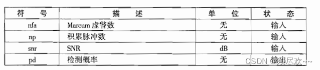
fig2_13.m

clear all
pfa = 1e-9;
nfa = log(2) / pfa;
index = 0;
for snr = -10:.5:30
   index = index +1;
   prob1(index) =  pd_swerling3 (nfa, 1, snr);
   prob10(index) =  pd_swerling3 (nfa, 10, snr);
   prob50(index) =  pd_swerling3(nfa, 50, snr);
   prob100(index) =  pd_swerling3 (nfa, 100, snr);
end
x = -10:.5:30;
plot(x, prob1,'k',x,prob10,'k:',x,prob50,'k--', ...
   x, prob100,'k-.');
axis([-10 30 0 1])
xlabel ('SNR - dB')
ylabel ('Probability of detection')
legend('np = 1','np = 10','np = 50','np = 100')
grid

2）仿真

检测概率相对于 SNR，Swerling Ⅲ， $P_{fa}=10^{-9}$
请添加图片描述
上图显示了当 $n_p=1，10，50，100$ 时，检测概率作为 SNR 函数的曲线，其中 $P_{fa}=10^{-9}$

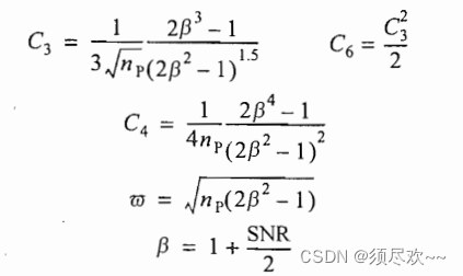
⑤、Swerling Ⅳ 型目标的检测

检测概率 $P_D$ ：
$n_p <50$ 时：
在这里插入图片描述
当 $n_p > 50$ 时：

此时：

1）MATLAB 源码

pd_swerling4.m

function pd = pd_swerling4 (nfa, np, snrbar)
% This function is used to calculate the probability of detection
% for Swerling 4 targets.
format long
snrbar = 10.0^(snrbar/10.);
eps = 0.00000001;
delmax = .00001;
delta =10000.;
% Calculate the threshold Vt
pfa =  np * log(2) / nfa;
sqrtpfa = sqrt(-log10(pfa));
sqrtnp = sqrt(np); 
vt0 = np - sqrtnp + 2.3 * sqrtpfa * (sqrtpfa + sqrtnp - 1.0);
vt = vt0;
while (abs(delta) >= vt0)
   igf = incomplete_gamma(vt0,np);
   num = 0.5^(np/nfa) - igf;
   temp = (np-1) * log(vt0+eps) - vt0 - factor(np-1);
   deno = exp(temp);
   vt = vt0 + (num / (deno+eps));
   delta = abs(vt - vt0) * 10000.0; 
   vt0 = vt;
end
h8 = snrbar /2.0;
beta = 1.0 + h8;
beta2 = 2.0 * beta^2 - 1.0;
beta3 = 2.0 * beta^3;
if (np >= 50)
   temp1 = 2.0 * beta -1;
   omegabar = sqrt(np * temp1);
   c3 = (beta3 - 1.) / 3.0 / beta2 / omegabar;
   c4 = (beta3 * beta3 - 1.0) / 4. / np /beta2 /beta2;;
   c6 = c3 * c3 /2.0;
   V = (vt - np * (1.0 + snrbar)) / omegabar;
   Vsqr = V *V;
   val1 = exp(-Vsqr / 2.0) / sqrt( 2.0 * pi);
   val2 = c3 * (V^2 -1.0) + c4 * V * (3.0 - V^2) - ... 
      c6 * V * (V^4 - 10. * V^2 + 15.0);
   q = 0.5 * erfc (V/sqrt(2.0));
   pd =  q - val1 * val2;
   return
else
   snr = 1.0;
   gamma0 = incomplete_gamma(vt/beta,np);
   a1 = (vt / beta)^np / (exp(factor(np)) * exp(vt/beta));
   sum = gamma0;
   for i = 1:1:np
      temp1 = 1;
      if (i == 1)
         ai = a1;
      else
         ai = (vt / beta) * a1 / (np + i -1);
      end
      a1 = ai;
      gammai = gamma0 - ai;
      gamma0 = gammai;
      a1 = ai;

      for ii = 1:1:i
         temp1 = temp1 * (np + 1 - ii);
      end
      term = (snrbar /2.0)^i * gammai * temp1 / exp(factor(i));
      sum = sum + term;
   end
   pd = 1.0 - sum / beta^np;
end
pd = max(pd,0.);

在这里插入图片描述

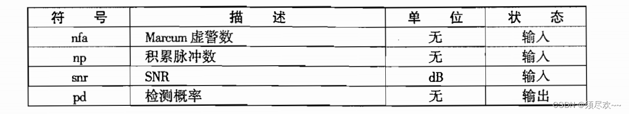
fig2_14.m

clear all
pfa = 1e-9;
nfa = log(2) / pfa;
index = 0;
for snr = -10:.5:30
   index = index +1;
   prob1(index) =  pd_swerling4 (nfa, 1, snr);
   prob10(index) =  pd_swerling4 (nfa, 10, snr);
   prob50(index) =  pd_swerling4(nfa, 50, snr);
   prob100(index) =  pd_swerling4 (nfa, 100, snr);
end
x = -10:.5:30;
plot(x, prob1,'k',x,prob10,'k:',x,prob50,'k--', ...
   x, prob100,'k-.');
axis([-10 30 0 1.1])
xlabel ('SNR - dB')
ylabel ('Probability of detection')
legend('np = 1','np = 10','np = 50','np = 100')
grid
axis tight