1.项目说明
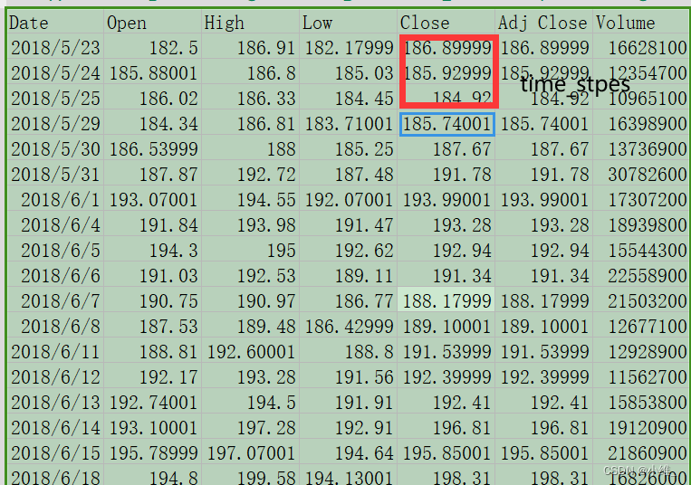
使用data中的close列的时间序列数据完成预测【使用close列数据中的前windowback-1天数据完成未来一天close的预测】
2.数据集
Date,Open,High,Low,Close,Adj Close,Volume
2018-05-23,182.500000,186.910004,182.179993,186.899994,186.899994,16628100
2018-05-24,185.880005,186.800003,185.029999,185.929993,185.929993,12354700
2018-05-25,186.020004,186.330002,184.449997,184.919998,184.919998,10965100
2018-05-29,184.339996,186.809998,183.710007,185.740005,185.740005,16398900
2018-05-30,186.539993,188.000000,185.250000,187.669998,187.669998,13736900
2018-05-31,187.869995,192.720001,187.479996,191.779999,191.779999,30782600
2018-06-01,193.070007,194.550003,192.070007,193.990005,193.990005,17307200
2018-06-04,191.839996,193.979996,191.470001,193.279999,193.279999,18939800
2018-06-05,194.300003,195.000000,192.619995,192.940002,192.940002,15544300
2018-06-06,191.029999,192.529999,189.110001,191.339996,191.339996,22558900
2018-06-07,190.750000,190.970001,186.770004,188.179993,188.179993,21503200
2018-06-08,187.529999,189.479996,186.429993,189.100006,189.100006,12677100
2018-06-11,188.809998,192.600006,188.800003,191.539993,191.539993,12928900
2018-06-12,192.169998,193.279999,191.559998,192.399994,192.399994,11562700
2018-06-13,192.740005,194.500000,191.910004,192.410004,192.410004,15853800
2018-06-14,193.100006,197.279999,192.910004,196.809998,196.809998,19120900
2018-06-15,195.789993,197.070007,194.639999,195.850006,195.850006,21860900
2018-06-18,194.800003,199.580002,194.130005,198.309998,198.309998,16826000
2018-06-19,196.240005,197.960007,193.789993,197.490005,197.490005,19994000
2018-06-20,199.100006,203.550003,198.809998,202.000000,202.000000,28230900
2018-06-21,202.759995,203.389999,200.089996,201.500000,201.500000,19045700
2018-06-22,201.160004,202.240005,199.309998,201.740005,201.740005,17420200
2018-06-25,200.000000,200.000000,193.110001,196.350006,196.350006,25275100
2018-06-26,197.600006,199.100006,196.229996,199.000000,199.000000,17897600
2018-06-27,199.179993,200.750000,195.800003,195.839996,195.839996,18734400
2018-06-28,195.179993,197.339996,193.259995,196.229996,196.229996,18172400
2018-06-29,197.320007,197.600006,193.960007,194.320007,194.320007,15811600
2018-07-02,193.369995,197.449997,192.220001,197.360001,197.360001,13961600
2018-07-03,194.550003,195.399994,192.520004,192.729996,192.729996,13489500
2018-07-05,194.740005,198.649994,194.029999,198.449997,198.449997,19684200
2018-07-06,198.449997,203.639999,197.699997,203.229996,203.229996,19740100
2018-07-09,204.929993,205.800003,202.119995,204.740005,204.740005,18149400
2018-07-10,204.500000,204.910004,202.259995,203.539993,203.539993,13190100
2018-07-11,202.220001,204.500000,201.750000,202.539993,202.539993,12927400
2018-07-12,203.429993,207.080002,203.190002,206.919998,206.919998,15454700
2018-07-13,207.809998,208.429993,206.449997,207.320007,207.320007,11486800
2018-07-16,207.500000,208.720001,206.839996,207.229996,207.229996,11078200
2018-07-17,204.899994,210.460007,204.839996,209.990005,209.990005,15349900
2018-07-18,209.820007,210.990005,208.440002,209.360001,209.360001,15334900
2018-07-19,208.770004,209.990005,207.759995,208.089996,208.089996,11350400
2018-07-20,208.850006,211.500000,208.500000,209.940002,209.940002,16163900
2018-07-23,210.580002,211.619995,208.800003,210.910004,210.910004,16732000
3.数据预处理
3.1 读取数据
ata = pd.read_csv('./data/rlData.csv')
data = data.sort_values('Date')
data.head()
data.shape

# 绘制close收盘价和Date时间的二维视图
sns.set_style("darkgrid")
plt.figure(figsize = (15,9))
plt.plot(data[['Close']])  #这里注意输入数据y的数据类型
plt.xticks(range(0,data.shape[0],20), data['Date'].loc[::20], rotation=45)
plt.title("****** Stock Price",fontsize=18, fontweight='bold')
plt.xlabel('Date',fontsize=18)
plt.ylabel('Close Price (USD)',fontsize=18)
plt.show()
3.2 选取特征工程Close列数据
price = data[['Close']]
price.info()
print(price.shape) #(25
3.3 数据归一化
scaler = MinMaxScaler(feature_range=(-1, 1))
price['Close'] = scaler.fit_transform(price['Close'].values.reshape(-1,1))
3.4 数据集的制造[batch_size,time_steps,input_size]
def split_data(stock, lookback):
    data_raw = stock.to_numpy()
    data = []
    # you can free play(seq_length)
    for index in range(len(data_raw) - lookback):

        #这里input的shape[252,1],然后每次取input中的[]
        """
        input= [[1],[2]...[252]]  input.shape=[252,1]
        每次循环取input[i:i+lookback],[[1],[2]...[lookback]] shape=[3,1]
        然后存到data列表中,经过若干次循环后就变成了【len(data_raw)-lookback,3,1】
        """
        data.append(data_raw[index: index + lookback])

    data = np.array(data)
    # print(data_raw.shape) #(252, 1)
    # print(data.shape)  #(249, 3, 1)


    test_set_size = int(np.round(0.2 * data.shape[0]))
    train_set_size = data.shape[0] - (test_set_size)

    x_train = data[:train_set_size,:-1,:] #当lookback=n时,本代码表示将time_step=n-1,其他数据不变
    y_train = data[:train_set_size,-1,:]  #当lookback=n时,本代码表示将n-1个数据作为y,且数据shape也会不变,和x_train保持一直

    x_test = data[train_set_size:,:-1,:]
    y_test = data[train_set_size:,-1,:]

    return [torch.Tensor(x_train), torch.Tensor(y_train), torch.Tensor(x_test),torch.Tensor(y_test)]

lookback = 3
x_train, y_train, x_test, y_test = split_data(price, lookback)
print('x_train.shape = ',x_train.shape) #(199, 2, 1)
print('y_train.shape = ',y_train.shape)
print('x_test.shape = ',x_test.shape) #x_test.shape =  (50, 2, 1)
print('y_test.shape = ',y_test.shape)
4.LSTM算法
class LSTM(nn.Module):
    def __init__(self, input_dim, hidden_dim, num_layers, output_dim):
        super(LSTM, self).__init__()
        self.hidden_dim = hidden_dim
        self.num_layers = num_layers

        self.lstm = nn.LSTM(input_dim, hidden_dim, num_layers, batch_first=True)
        self.fc = nn.Linear(hidden_dim, output_dim)

    def forward(self, x):
        """
        batch_first=True:则输入为x.shape = (batch_size,time_steps,input_size)
                                out.shape = (batch_size,time-steps,ouput_size)

        """
        h0 = torch.zeros(self.num_layers, x.size(0), self.hidden_dim).requires_grad_()
        c0 = torch.zeros(self.num_layers, x.size(0), self.hidden_dim).requires_grad_()

        # x.shape = (batch_size,time_steps,input_size)
        # out.shape = (batch_size,time_steps,ouput_size)
        out, (hn, cn) = self.lstm(x, (h0.detach(), c0.detach()))

        #out.shape是选取time_steps列的最后一个数据 out.shape = (batch_size,ouput_size)
        out = self.fc(out[:, -1, :])
        return out
5.预训练
input_dim = 1
hidden_dim = 32
num_layers = 2
output_dim = 1
num_epochs = 100

model = LSTM(input_dim=input_dim, hidden_dim=hidden_dim, output_dim=output_dim, num_layers=num_layers)
criterion = torch.nn.MSELoss()
optimiser = torch.optim.Adam(model.parameters(), lr=0.01)


hist = np.zeros(num_epochs)
lstm = []

for t in range(num_epochs):

    #x_train.shape=torch.Size([199, 2, 1])     [batch_size,time_steps,input_size]
    #y_train_pred.shape=torch.Size([199, 1])   [batch_size,ouput_size]

    y_train_pred = model(x_train)

    loss = criterion(y_train_pred, y_train_lstm)
    # print("Epoch ", t, "MSE: ", loss.item())
    hist[t] = loss.item()

    optimiser.zero_grad()
    loss.backward()
    optimiser.step()
6.绘制预测值和真实值拟合图形,以及loss图形
#绘制预测值y_train_pred和真实值y_train二维视图
predict = pd.DataFrame(scaler.inverse_transform(y_train_pred.detach().numpy()))
original = pd.DataFrame(scaler.inverse_transform(y_train.detach().numpy()))


sns.set_style("darkgrid")
fig = plt.figure()
fig.subplots_adjust(hspace=0.2, wspace=0.2)

plt.subplot(1, 2, 1)
ax = sns.lineplot(x = original.index, y = original[0], label="Data", color='royalblue')
ax = sns.lineplot(x = predict.index, y = predict[0], label="Training Prediction (LSTM)", color='tomato')
ax.set_title('Stock price', size = 14, fontweight='bold')
ax.set_xlabel("Days", size = 14)
ax.set_ylabel("Cost (USD)", size = 14)
ax.set_xticklabels('', size=10)

plt.subplot(1, 2, 2)
ax = sns.lineplot(data=hist, color='royalblue')
ax.set_xlabel("Epoch", size = 14)
ax.set_ylabel("Loss", size = 14)
ax.set_title("Training Loss", size = 14, fontweight='bold')
fig.set_figheight(6)
fig.set_figwidth(16)
7.测试集测试
model.eval()

# make predictions
y_test_pred = model(x_test)

# invert predictions
y_train_pred = scaler.inverse_transform(y_train_pred.detach().numpy())
y_train = scaler.inverse_transform(y_train.detach().numpy())
y_test_pred = scaler.inverse_transform(y_test_pred.detach().numpy())
y_test = scaler.inverse_transform(y_test.detach().numpy())

# calculate root mean squared error
trainScore = math.sqrt(mean_squared_error(y_train[:,0], y_train_pred[:,0]))
print('Train Score: %.2f RMSE' % (trainScore))
testScore = math.sqrt(mean_squared_error(y_test[:,0], y_test_pred[:,0]))
print('Test Score: %.2f RMSE' % (testScore))
lstm.append(trainScore)
lstm.append(testScore)
lstm.append(training_time)
完整代码
import numpy as np
import pandas as pd
import matplotlib.pyplot as plt
import seaborn as sns
from sklearn.preprocessing import MinMaxScaler
import torch
import torch.nn as nn
import time
import math, time
from sklearn.metrics import mean_squared_error
import seaborn as sns

data = pd.read_csv('./data/rlData.csv')
data = data.sort_values('Date')
data.head()
data.shape

# 绘制close收盘价和Date时间的二维视图
sns.set_style("darkgrid")
plt.figure(figsize = (15,9))
plt.plot(data[['Close']])  #这里注意输入数据y的数据类型
plt.xticks(range(0,data.shape[0],20), data['Date'].loc[::20], rotation=45)
plt.title("****** Stock Price",fontsize=18, fontweight='bold')
plt.xlabel('Date',fontsize=18)
plt.ylabel('Close Price (USD)',fontsize=18)
plt.show()


#1.选取特征工程Close类数据
price = data[['Close']]
price.info()
print(price.shape) #(252, 1)

#2.数据归一化
scaler = MinMaxScaler(feature_range=(-1, 1))
price['Close'] = scaler.fit_transform(price['Close'].values.reshape(-1,1))

#3.数据集的制作
def split_data(stock, lookback):
    data_raw = stock.to_numpy()
    data = []
    # you can free play(seq_length)
    for index in range(len(data_raw) - lookback):

        #这里input的shape[252,1],然后每次取input中的[]
        """
        input= [[1],[2]...[252]]  input.shape=[252,1]
        每次循环取input[i:i+lookback],[[1],[2]...[lookback]] shape=[3,1]
        然后存到data列表中,经过若干次循环后就变成了【len(data_raw)-lookback,3,1】
        """
        data.append(data_raw[index: index + lookback])

    data = np.array(data)
    # print(data_raw.shape) #(252, 1)
    # print(data.shape)  #(249, 3, 1)


    test_set_size = int(np.round(0.2 * data.shape[0]))
    train_set_size = data.shape[0] - (test_set_size)

    x_train = data[:train_set_size,:-1,:] #当lookback=n时,本代码表示将time_step=n-1,其他数据不变
    y_train = data[:train_set_size,-1,:]  #当lookback=n时,本代码表示将n-1个数据作为y,且数据shape也会不变,和x_train保持一直

    x_test = data[train_set_size:,:-1,:]
    y_test = data[train_set_size:,-1,:]

    return [torch.Tensor(x_train), torch.Tensor(y_train), torch.Tensor(x_test),torch.Tensor(y_test)]

lookback = 3
x_train, y_train, x_test, y_test = split_data(price, lookback)
print('x_train.shape = ',x_train.shape) #(199, 2, 1)
print('y_train.shape = ',y_train.shape)
print('x_test.shape = ',x_test.shape) #x_test.shape =  (50, 2, 1)
print('y_test.shape = ',y_test.shape)

class LSTM(nn.Module):
    def __init__(self, input_dim, hidden_dim, num_layers, output_dim):
        super(LSTM, self).__init__()
        self.hidden_dim = hidden_dim
        self.num_layers = num_layers

        self.lstm = nn.LSTM(input_dim, hidden_dim, num_layers, batch_first=True)
        self.fc = nn.Linear(hidden_dim, output_dim)

    def forward(self, x):
        """
        batch_first=True:则输入为x.shape = (batch_size,time_steps,input_size)
                                out.shape = (batch_size,time-steps,ouput_size)

        """
        h0 = torch.zeros(self.num_layers, x.size(0), self.hidden_dim).requires_grad_()
        c0 = torch.zeros(self.num_layers, x.size(0), self.hidden_dim).requires_grad_()

        # x.shape = (batch_size,time_steps,input_size)
        # out.shape = (batch_size,time_steps,ouput_size)
        out, (hn, cn) = self.lstm(x, (h0.detach(), c0.detach()))

        #out.shape是选取time_steps列的最后一个数据 out.shape = (batch_size,ouput_size)
        out = self.fc(out[:, -1, :])
        return out

input_dim = 1
hidden_dim = 32
num_layers = 2
output_dim = 1
num_epochs = 100

model = LSTM(input_dim=input_dim, hidden_dim=hidden_dim, output_dim=output_dim, num_layers=num_layers)
criterion = torch.nn.MSELoss()
optimiser = torch.optim.Adam(model.parameters(), lr=0.01)


hist = np.zeros(num_epochs)
lstm = []

for t in range(num_epochs):

    #x_train.shape=torch.Size([199, 2, 1])     [batch_size,time_steps,input_size]
    #y_train_pred.shape=torch.Size([199, 1])   [batch_size,ouput_size]

    y_train_pred = model(x_train)

    loss = criterion(y_train_pred, y_train_lstm)
    # print("Epoch ", t, "MSE: ", loss.item())
    hist[t] = loss.item()

    optimiser.zero_grad()
    loss.backward()
    optimiser.step()

#绘制预测值y_train_pred和真实值y_train二维视图
predict = pd.DataFrame(scaler.inverse_transform(y_train_pred.detach().numpy()))
original = pd.DataFrame(scaler.inverse_transform(y_train.detach().numpy()))


sns.set_style("darkgrid")
fig = plt.figure()
fig.subplots_adjust(hspace=0.2, wspace=0.2)

plt.subplot(1, 2, 1)
ax = sns.lineplot(x = original.index, y = original[0], label="Data", color='royalblue')
ax = sns.lineplot(x = predict.index, y = predict[0], label="Training Prediction (LSTM)", color='tomato')
ax.set_title('Stock price', size = 14, fontweight='bold')
ax.set_xlabel("Days", size = 14)
ax.set_ylabel("Cost (USD)", size = 14)
ax.set_xticklabels('', size=10)

plt.subplot(1, 2, 2)
ax = sns.lineplot(data=hist, color='royalblue')
ax.set_xlabel("Epoch", size = 14)
ax.set_ylabel("Loss", size = 14)
ax.set_title("Training Loss", size = 14, fontweight='bold')
fig.set_figheight(6)
fig.set_figwidth(16)


# 设置成eval模式
model.eval()

# make predictions
y_test_pred = model(x_test)

# invert predictions
y_train_pred = scaler.inverse_transform(y_train_pred.detach().numpy())
y_train = scaler.inverse_transform(y_train.detach().numpy())
y_test_pred = scaler.inverse_transform(y_test_pred.detach().numpy())
y_test = scaler.inverse_transform(y_test.detach().numpy())

# calculate root mean squared error
trainScore = math.sqrt(mean_squared_error(y_train[:,0], y_train_pred[:,0]))
print('Train Score: %.2f RMSE' % (trainScore))
testScore = math.sqrt(mean_squared_error(y_test[:,0], y_test_pred[:,0]))
print('Test Score: %.2f RMSE' % (testScore))
lstm.append(trainScore)
lstm.append(testScore)
lstm.append(training_time)
参考:https://gitee.com/qiangchen_sh/stock-prediction/blob/master/%E4%BB%A3%E7%A0%81/LSTM%E4%BB%8E%E7%90%86%E8%AE%BA%E5%9F%BA%E7%A1%80%E5%88%B0%E4%BB%A3%E7%A0%81%E5%AE%9E%E6%88%98%203%20%E8%82%A1%E7%A5%A8%E4%BB%B7%E6%A0%BC%E9%A2%84%E6%B5%8B_Pytorch.ipynb#