捕食者与猎物模型
人口增长
在人口增长或衰减的最简单模型中,增长速度或衰减速度与人口本身的数目成正比。增加或减少人口规模会导致出生和死亡数量成比例地增加或减少。在数学上,可以由以下微分方程描述。
可以得出:,其中
。
该简单模型在人口增长的初始阶段是正确的,因为初始阶段对人口没有限制。在现实情况下,人口数量增加时,其增长速度按照线性方式下降。这个微分方程模型有时称为logistic方程。
新参数μ为承载能力,当y(t)接近于μ,增长率接近于0,人口增长逐渐停止。
%% Exponential and Logistic Growth.采用指数增长和logistic增长
   close all
   figure
   k = 1
   eta = 1
   mu = 20
   t = 0:1/32:8;
   y = mu*eta*exp(k*t)./(eta*exp(k*t) + mu - eta);
   plot(t,[y; exp(t)])
   axis([0 8 0 22])
   title('Exponential and logistic growth')
   xlabel('t')
   ylabel('y')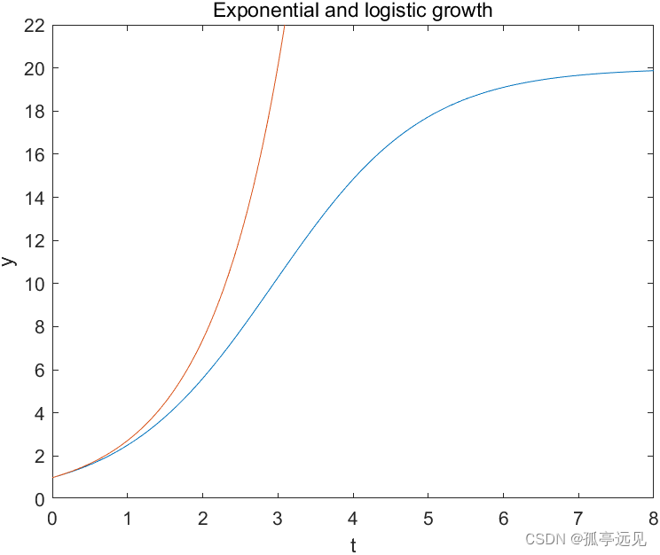
或采用ode45来求常微分方程组的数值解:
%% ODE45 for the Logistic Model.
   figure
   k = 1
   eta = 1
   mu = 20
   ydot = @(t,y) k*(1-y/mu)*y
   ode45(ydot,[0 8],eta)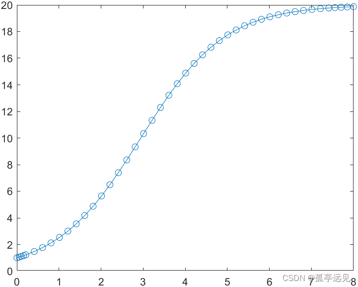
在使用ode45求解时,@符号和@(t,y)可以定义出t和y的函数。变量t必须给出,即使某个微分方程像这里的方程那样不显含时间变量t。
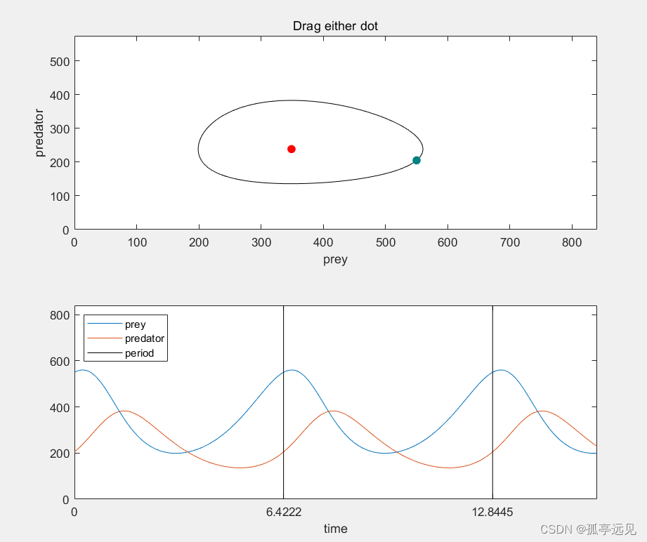
捕食者与猎物模型
捕食者和猎物模型为两个方程,这设计两个竞争物种y1(t)和y2(t)的变化情况。y1的增长率是y2的现象函数,反过来也是。
单物种logistic模型是有求解公式的,但对捕食者与猎物模型来说,不能得出包括指数函数、三角函数或其他基本函数的解析解,这时只能求出方程的数值解。
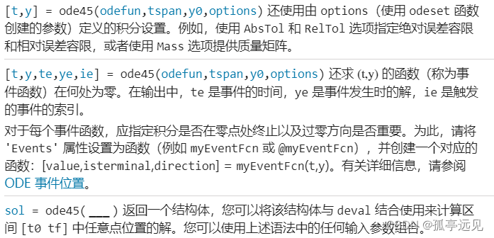
ode45
function predprey(action)
% PREDPREY  Predator-prey gui.
% Drag the red dot to change equilibrium point.
% Drag the blue-green dot to change the initial conditions.

   % Default parameters.

   mu = [300 200]';     % Equilibrium.
   eta = [400 100]';    % Initial conditions.

   % Predator-prey ode

   function ydot = ppode(t,y);
      ydot = [(1-y(2)/mu(2))*y(1);
             -(1-y(1)/mu(1))*y(2)];
   end

   % Switchyard.

   if nargin == 0
      action = 'init';
   end
   switch action
      case 'init'
         initialize_graphics
      case 'down'
         locate_dot
         return
      case 'move'
         move_dot
      case 'up'
         free_dot
   end

   % Solve ode.

   [mu, eta] = get_parameters;
   opts = odeset('reltol',1.e-8,'events',@pitstop);
   [t,y,te] = ode45(@ppode,[0 100],eta,opts);

   % Update the plots.

   subplot1(y,action)
   subplot2(t,y,te,action)

   % ----------------------------------

   function [g,isterm,dir] = pitstop(t,y)
      % Event function called by the ode solver.
      % Terminate when y returns to the point where its angle
      % with mu is the same as the angle between eta and mu.
      sig = sign(eta(1)-mu(1)+realmin);
      theta1 = atan2(sig*(y(2)-mu(2)),sig*(y(1)-mu(1)));
      theta0 = atan2(sig*(eta(2)-mu(2)),sig*(eta(1)-mu(1)));
      g = theta1 - theta0;
      isterm = t > 1;
      dir = 1;
   end

   % ----------------------------------

   function initialize_graphics  %初始化图形
      % Set up two subplots, buttons, dots and empty plots.
      clf
      shg
      set(gcf,'units','normal','pos',[.25 .125 .50 .75])
      subplot(2,1,1)
      plot(0,0,'-','color','black');
      line(mu(1),mu(2),'marker','.','markersize',24,'color',[1 0 0]);
      line(eta(1),eta(2),'marker','.','markersize',24,'color',[0 1/2 1/2]);
      xlabel('prey')
      ylabel('predator')
      title('Drag either dot')
      subplot(2,1,2)
      plot(0,[0 0]);
      line([0 0],[0 0],'color','black');
      line([0 0],[0 0],'color','black');
      xlabel('time')
      legend('prey','predator','period','location','northwest')
      set(gcf,'windowbuttondownfcn','predprey(''down'')', ...
              'windowbuttonmotionfcn','predprey(''move'')', ...
              'windowbuttonupfcn','predprey(''up'')')
      set(gcf,'userdata',[])
   end

   % ----------------------------------

   function locate_dot
      % Find if the mouse is selecting one of the dots.
      point = get(gca,'currentpoint');
      h = get(gca,'children');
      y1 = get(h(1:2),'xdata');
      y2 = get(h(1:2),'ydata');
      d = abs([y1{:}]'-point(1,1)) + abs([y2{:}]'-point(1,2));
      k = min(find(d == min(d)));
      tol = .025*max(abs(axis));
      if d(k) < tol
         set(gcf,'userdata',h(k))
      else
         set(gcf,'userdata',[])
      end
   end

   % ----------------------------------

   function move_dot
      % Move the selected dot to a new position.
      point = abs(get(gca,'currentpoint'));
      hit = get(gcf,'userdata');
      if ~isempty(hit)
         set(hit,'xdata',point(1,1),'ydata',point(1,2))
      end
   end

   % ----------------------------------

   function free_dot
      % Deselect the dot.
      set(gcf,'userdata',[])
   end

   % ----------------------------------

   function [mu,eta] = get_parameters
      % Obtain mu and eta from the two dots.
      subplot(2,1,1);
      h = get(gca,'children');
      mu = [get(h(2),'xdata') get(h(2),'ydata')]';
      eta = [get(h(1),'xdata') get(h(1),'ydata')]';
   end

   % ----------------------------------

   function subplot1(y,action)
      % Redraw the phase plane plot and perhaps rescale.
      subplot(2,1,1)
      h = get(gca,'children');
      set(h(3),'xdata',y(:,1),'ydata',y(:,2));
      if ~isequal(action,'move')
         y1max = max(max(y(:,1)),mu(1));
         y2max = max(max(y(:,2)),mu(2));
         axis([0 1.5*y1max 0 1.5*y2max])
      end
   end

   % ----------------------------------

   function subplot2(t,y,te,action)
      % Redraw the time plots, period line, and perhaps rescale.
      subplot(2,1,2)
      if length(te)==0 || te(end) < 1.e-6
         pit = 2*pi;
      else
         pit = te(end);
      end
      h = get(gca,'children');
      ymax = max(max(y));
      t = [t; t+pit; t+2*pit];
      y = [y; y; y];
      set(h(4),'xdata',t,'ydata',y(:,1));
      set(h(3),'xdata',t,'ydata',y(:,2));
      set(h(2),'xdata',[pit pit],'ydata',[0 3*ymax]);
      set(h(1),'xdata',[2*pit 2*pit],'ydata',[0 3*ymax]);
      set(gca,'xtick',[0 pit 2*pit])
      if ~isequal(action,'move')
         axis([0 2.5*pit 0 1.5*ymax])
      end
      subplot(2,1,1)
   end
end
轨道
轨道是多天体系统的动力学问题。
弹跳球模型
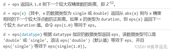
eps
在初始时刻小球上抛之后,地球的引力是的速度每步都按照固定的比率g减少。
%% Core of bouncer, simple gravity. no gravity

   % Initialize

   z0 = eps;
   g = 9.8;
   c = 0.75;
   delta = 0.005;
   v0 = 21;
   y = [];

   % Bounce

   while v0 >= 1
      v = v0;
      z = z0;
      while z >= 0
         v = v - delta*g;
         z = z + delta*v;
         y = [y  z];
      end
      v0 = c*v0;
   end

   % Simplified graphics

   close all
   figure
   plot(y)
布朗运动
随机游走(random walk)的简单布朗运动
%% Snapshot of two dimensional Brownian motion.
figure
m = 100;
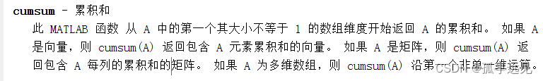
x = cumsum(randn(m,1));
y = cumsum(randn(m,1));
plot(x,y,'.-')
s = 2*sqrt(m);
axis([-s s -s s]);
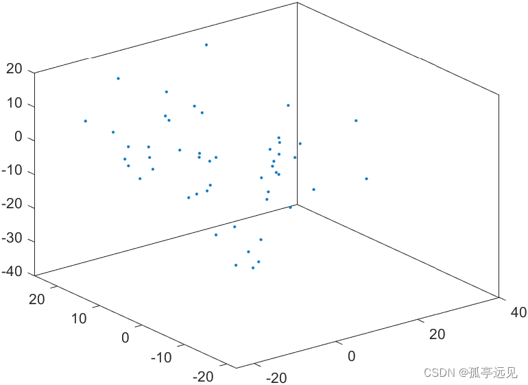
%% Snapshot of three dimensional Brownian motion, brownian3
n = 50; %粒子个数
delta = 0.125;
P = zeros(n,3);
for t = 0:10000
% Normally distributed random velocities.生成正态分布的随机速度
V = randn(n,3);
% Update positions. 更新位置
P = P + delta*V;
end
figure
plot3(P(:,1),P(:,2),P(:,3),'.')
box on

n天体问题
(1)前向法(显式欧拉法)
(2)后向法(隐式欧拉法)
(3)耦对法(前两种方法的折中)
function orbits(n,gui)
% ORBITS n-body gravitational attraction for n = 2, 3 or 9.
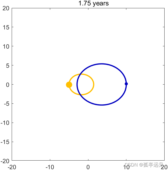
% ORBITS(2), two bodies, classical elliptic orbits.
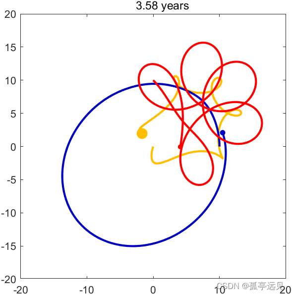
% ORBITS(3), three bodies, artificial planar orbits.
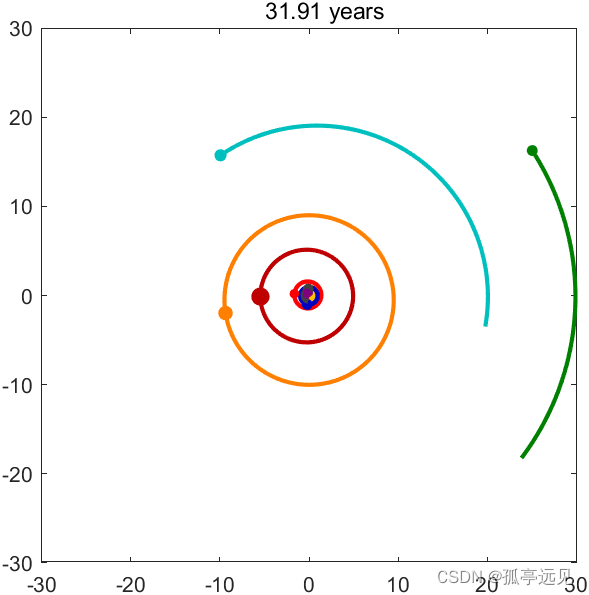
% ORBITS(9), nine bodies, the solar system with one sun and 8 planets.
%
% ORBITS(n,false) turns off the uicontrols and generates a static plot.
% ORBITS(n,false) 关闭 uicontrols 并生成静态图。
% ORBITS with no arguments is the same as ORBITS(9,true).
% n = number of bodies.
% P = n-by-3 array of position coordinates.
% V = n-by-3 array of velocities
% M = n-by-1 array of masses
% H = graphics and user interface handles
if (nargin < 2)
gui = true;
end
if (nargin < 1);
n = 9;
end
[P,V,M] = initialize_orbits(n);
H = initialize_graphics(P,gui);
steps = 20; % Number of steps between plots
t = 0; % time
while get(H.stop,'value') == 0
% Obtain step size from slider.
delta = get(H.speed,'value')/(20*steps);
for k = 1:steps
% Compute current gravitational forces.
G = zeros(size(P));
for i = 1:n
for j = [1:i-1 i+1:n];
r = P(j,:) - P(i,:);
G(i,:) = G(i,:) + M(j)*r/norm(r)^3;
end
end
% Update velocities using current gravitational forces.
V = V + delta*G;
% Update positions using updated velocities.
P = P + delta*V;
end
t = t + steps*delta;
H = update_plot(P,H,t,gui);
end
finalize_graphics(H,gui)
end
%% Inialize orbits ---------------------------------------------------
function [P,V,M] = initialize_orbits(n)
switch n
%% Two bodies
case 2
% Initial position, velocity, and mass for two bodies.
% Resulting orbits are ellipses.
P = [-5 0 0
10 0 0];
V = [ 0 -1 0
0 2 0];
M = [200 100 0];
%% Three bodies
case 3
% Initial position, velocity, and mass for the artificial
% planar three body problem discussed in the text.
P = [ 0 0 0
10 0 0
0 10 0];
V = [-1 -3 0
0 6 0
3 -3 0];
M = [300 200 100]';
%% Nine bodies
case 9
% The solar system.
% Obtain data from Jet Propulsion Laboratory HORIZONS.
% http://ssd.jpl.nasa.gov/horizons.cgi
% Ephemeris Type: VECTORS
% Coordinate Orgin: Sun (body center)
% Time Span: 2008-7-24 to 2008-7-25
sol.p = [0 0 0];
sol.v = [0 0 0];
sol.m = 1.9891e+30;
ear.p = [ 5.28609710e-1 -8.67456608e-1 1.28811732e-5];
ear.v = [ 1.44124476e-2 8.88154404e-3 -6.00575229e-7];
ear.m = 5.9736e+24;
mar.p = [-1.62489742e+0 -2.24489575e-1 3.52032835e-2];
mar.v = [ 2.43693131e-3 -1.26669231e-2 -3.25240784e-4];
mar.m = 6.4185e+23;
mer.p = [-1.02050180e-2 3.07938393e-1 2.60947941e-2];
mer.v = [-3.37623365e-2 9.23226497e-5 3.10568978e-3];
mer.m = 3.302e+23;
ven.p = [-6.29244070e-1 3.44860019e-1 4.10363705e-2];
ven.v = [-9.80593982e-3 -1.78349270e-2 3.21808697e-4];
ven.m = 4.8685e+24;
jup.p = [ 1.64800250e+0 -4.90287752e+0 -1.65248109e-2];
jup.v = [ 7.06576969e-3 2.76492888e-3 -1.69566833e-4];
jup.m = 1.8986e+27;
sat.p = [-8.77327303e+0 3.13579422e+0 2.94573194e-1];
sat.v = [-2.17081741e-3 -5.26328586e-3 1.77789483e-4];
sat.m = 5.6846e+26;
ura.p = [ 1.97907257e+1 -3.48999512e+0 -2.69289277e-1];
ura.v = [ 6.59740515e-4 3.69157117e-3 5.11221503e-6];
ura.m = 8.6832e+25;
nep.p = [ 2.38591173e+1 -1.82478542e+1 -1.74095745e-1];
nep.v = [ 1.89195404e-3 2.51313400e-3 -9.54022068e-5];
nep.m = 1.0243e+26;
P = [sol.p; ear.p; mar.p; mer.p; ven.p; jup.p; sat.p; ura.p; nep.p];
V = [sol.v; ear.v; mar.v; mer.v; ven.v; jup.v; sat.v; ura.v; nep.v];
M = [sol.m; ear.m; mar.m; mer.m; ven.m; jup.m; sat.m; ura.m; nep.m];
% Scale mass by solar mass.
M = M/sol.m;
% Scale velocity to radians per year.
V = V*365.25/(2*pi);
% Adjust sun's initial velocity so that system total momentum is zero.
V(1,:) = -sum(diag(M)*V);
otherwise
error('No initial data for %d bodies',n)
end % switch
end
%% Initialize graphics --------------------------------------
function H = initialize_graphics(P,gui)
% Initialize graphics and user interface controls
% H = initialize_graphics(P,gui)
% H = handles, P = positions, gui = true or false for gui or static plot.
dotsize = [36 18 16 12 18 30 24 20 18]';
color = [4 3 0 % gold
0 0 3 % blue
4 0 0 % red
2 0 2 % magenta
1 1 1 % gray
3 0 0 % dark red
4 2 0 % orange
0 3 3 % cyan
0 2 0]/4; % dark green
clf reset
n = size(P,1);
s = max(sqrt(diag(P*P')));
if n <= 3, s = 2*s; end
axis([-s s -s s -s/4 s/4])
axis square
if n <= 3, view(2), end
box on
for i = 1:n
H.bodies(i) = line(P(i,1),P(i,2),P(i,3),'color',color(i,:), ...
'marker','.','markersize',dotsize(i),'userdata',dotsize(i));
end
H.clock = title('0 years','fontweight','normal');
H.stop = uicontrol('string','stop','style','toggle', ...
'units','normal','position',[.90 .02 .08 .04]);
if n < 9
maxsp = 0.5;
else
maxsp = 10;
end
if gui
H.speed = uicontrol('style','slider','min',0,'value',maxsp/4, ...
'max',maxsp,'units','normal','position',[.02 .02 .30 .04], ...
'sliderstep',[1/20 1/20]);
uicontrol('string','trace','style','toggle','units','normal', ...
'position',[.34 .02 .06 .04],'callback','tracer');
uicontrol('string','in','style','pushbutton','units','normal', ...
'position',[.42 .02 .06 .04],'callback','zoomer(1/sqrt(2))')
uicontrol('string','out','style','pushbutton','units','normal', ...
'position',[.50 .02 .06 .04],'callback','zoomer(sqrt(2))')
uicontrol('string','x','style','pushbutton','units','normal', ...
'position',[.58 .02 .06 .04],'callback','view(0,0)')
uicontrol('string','y','style','pushbutton','units','normal', ...
'position',[.66 .02 .06 .04],'callback','view(90,0)')
uicontrol('string','z','style','pushbutton','units','normal', ...
'position',[.74 .02 .06 .04],'callback','view(0,90)')
uicontrol('string','3d','style','pushbutton','units','normal', ...
'position',[.82 .02 .06 .04],'callback','view(-37.5,30)')
else
H.traj = P;
H.speed = uicontrol('value',maxsp,'vis','off');
end
set(gcf,'userdata',H)
drawnow
end
%% Tracer ----------------------------------------------------------
function tracer
% Callback for trace button
H = get(gcf,'userdata');
bodies = flipud(H.bodies);
trace = get(gcbo,'value');
n = length(bodies);
for i = 1:n
if trace
ms = 6;
if n == 9 && i == 1, ms = 24; end
set(bodies(i),'markersize',ms,'erasemode','none')
else
ms = get(bodies(i),'userdata');
set(bodies(i),'markersize',ms,'erasemode','normal')
end
end
if trace
set(H.clock,'erasemode','xor')
else
set(H.clock,'erasemode','normal')
end
end
%% Zoomer ---------------------------------------------------
function zoomer(zoom)
% Callback for in and out buttons
H = get(gcf,'userdata');
[az,el] = view;
view(3);
axis(zoom*axis);
view(az,el);
set(H.speed,'max',zoom*get(H.speed,'max'), ...
'value',zoom*get(H.speed,'value'));
end
%% Update plot ------------------------------------------------
function H = update_plot(P,H,t,gui)
set(H.clock,'string',sprintf('%10.2f years',t/(2*pi)))
for i = 1:size(P,1)
set(H.bodies(i),'xdata',P(i,1),'ydata',P(i,2),'zdata',P(i,3))
end
if ~gui
H.traj(:,:,end+1) = P;
n = size(H.traj,1);
switch n
case 2, set(H.stop,'value',t > 11)
case 3, set(H.stop,'value',t > 22.5)
case 9, set(H.stop,'value',t > 200)
end
end
drawnow
end
%% Finalize graphics -------------------------------------------
function finalize_graphics(H,gui)
delete(findobj('type','uicontrol'))
uicontrol('string','close','style','pushbutton', ...
'units','normal','position',[.90 .02 .08 .04],'callback','close');
if ~gui
n = size(H.traj,1);
for i = 1:n
line(squeeze(H.traj(i,1,:)),squeeze(H.traj(i,2,:)), ...
squeeze(H.traj(i,3,:)),'color',get(H.bodies(i),'color'), ...
'linewidth',2)
end
end
end
%% Run all three orbits, with 2, 3, and 9 bodies, and no gui.

   figure
   orbits(2,false)

   figure
   orbits(3,false)

   figure
   orbits(9,false)