泰勒图（Taylor diagram）

泰勒图是Karl E. Taylor于2001年首先提出，主要用来比较几个气象模式模拟的能力，因此该表示方法在气象领域使用最多，但是在其他自然科学领域也有一定的应用。
泰勒图常用于评价模型的精度，常用的精度指标有相关系数（correlation coefficient），标准差（standard deviation）以及中心均方根误差（centered root-mean-square, RMSE）。
一般而言，泰勒图中的散点代表模型，辐射线代表相关系数，横纵轴代表标准差，而虚线代表均方根误差。泰勒图一改以往用散点图这种只能呈现两个指标来表示模型精度的情况。
泰勒图分为标准化泰勒图和未标准化泰勒图，用的比较多的是标准化泰勒图。标准化泰勒图即对参考值与变量值的标准差与均方根误差同除以参考值的标准差，令参考值=1，E=0，并消除其物理量单位。

泰勒图基本介绍

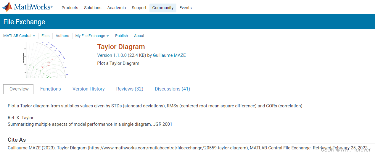
1 绘制包下载

安装网站：Taylor Diagram
在这里插入图片描述
Google Code Archive
此外，还需要"allstats"和"ptable"函数，下载链接分别如下：
Github-allstats.m函数

% STATM Compute statistics from 2 series
%
% STATM = allstats(Cr,Cf)
%
% Compute statistics from 2 series considering Cr as the reference.
% 
% Inputs:
%	Cr and Cf are of same length and uni-dimensional. They may contain NaNs.
%
% Outputs:
% 	STATM(1,:) => Mean
% 	STATM(2,:) => Standard Deviation (scaled by N)
% 	STATM(3,:) => Centered Root Mean Square Difference (scaled by N)
% 	STATM(4,:) => Correlation
%
% Notes:
%	- N is the number of points where BOTH Cr and Cf are defined
%
% 	- NaN are handled in the following way: because this function
% 		aims to compair 2 series, statistics are computed with indices
%		where both Cr and Cf are defined.
%
% 	- STATM(:,1) are from Cr (ie with C=Cr hereafter)
% 	  STATM(:,2) are from Cf versus Cr (ie with C=Cf hereafter)
%
%	- The MEAN is computed using the Matlab mean function.
%
%	- The STANDARD DEVIATION is computed as:
%			          /  sum[ {C-mean(C)} .^2]  \
%			STD = sqrt|  ---------------------  |
%			          \          N              /
%
%	- The CENTERED ROOT MEAN SQUARE DIFFERENCE is computed as:
%			           /  sum[  { [C-mean(C)] - [Cr-mean(Cr)] }.^2  ]  \
%			RMSD = sqrt|  -------------------------------------------  |
%			           \                      N                        /
%
%	- The CORRELATION is computed as:
%			      sum( [C-mean(C)].*[Cr-mean(Cr)] ) 
%			COR = --------------------------------- 
%			              N*STD(C)*STD(Cr)
%
%	- STATM(3,1) = 0 and STATM(4,1) = 1 by definition !
%
% Created by Guillaume Maze on 2008-10-28.
% Rev. by Guillaume Maze on 2010-02-10: Add NaN values handling, some checking
%				in the inputs and a more complete help
% Copyright (c) 2008 Guillaume Maze. 
% http://codes.guillaumemaze.org




%
% This program is free software: you can redistribute it and/or modify it under the terms of the GNU General Public License as published by
% the Free Software Foundation, either version 3 of the License, or any later version.
% This program is distributed in the hope that it will be useful, but WITHOUT ANY WARRANTY; without even the implied warranty of
% MERCHANTABILITY or FITNESS FOR A PARTICULAR PURPOSE.  See the GNU General Public License for more details.
% You should have received a copy of the GNU General Public License along with this program.  If not, see <http://www.gnu.org/licenses/>.
%

function STATM = allstats(varargin)
	
Cr = varargin{1}; Cr = Cr(:);
Cf = varargin{2}; Cf = Cf(:);

%%% Check size:
if length(Cr) ~= length(Cf)
	error('Cr and Cf must be of same length');
end

%%% Check NaNs:
iok = find(isnan(Cr)==0 & isnan(Cf)==0);
if length(iok) ~= length(Cr)
	warning('Found NaNs in inputs, removed them to compute statistics');
end
Cr  = Cr(iok);
Cf  = Cf(iok);
N   = length(Cr);

%%% STD:
st(1) = sqrt(sum(  (Cr-mean(Cr) ).^2)  / N );
st(2) = sqrt(sum(  (Cf-mean(Cf) ).^2)  / N );
%st(1) = sqrt(sum(  (Cr-mean(Cr) ).^2)  / (N-1) );
%st(2) = sqrt(sum(  (Cf-mean(Cf) ).^2)  / (N-1) );

%%% MEAN:
me(1) = mean(Cr);
me(2) = mean(Cf);

%%% RMSD:
rms(1) = sqrt(sum(  ( ( Cr-mean(Cr) )-( Cr-mean(Cr) )).^2)  /N);
rms(2) = sqrt(sum(  ( ( Cf-mean(Cf) )-( Cr-mean(Cr) )).^2)  /N);

%%% CORRELATIONS:
co(1) = sum(  ( ( Cr-mean(Cr) ).*( Cr-mean(Cr) )))/N/st(1)/st(1);
co(2) = sum(  ( ( Cf-mean(Cf) ).*( Cr-mean(Cr) )))/N/st(2)/st(1);


%%% OUTPUT
STATM(1,:) = me;
STATM(2,:) = st;
STATM(3,:) = rms;
STATM(4,:) = co;
	
end %function

Github-ptable.m函数
ptable.m函数如下：

% PTABLE Creates non uniform subplot handles
%
% SUBPLOT_HANDLE = ptable(TSIZE,PCOORD)
%
% This function creates subplot handles according to
% TSIZE and PCOORD.
% TSIZE(2) is the underlying TABLE of subplots: TSIZE(1)
%	is the number of lines, TSIZE(2) the number of rows
% PCOORD(:,2) indicates the coordinates of the subplots, ie
% 	for each PCOORD(i,2), the subplot i extends from
%	initial subplot PCOORD(i,1) to subplot PCOORD(i,2)
%
% Example: 
%	figure
% 	subp = ptable([3 4],[1 6 ; 3 4 ; 9 11; 8 8]);
%	x = 0:pi/180:2*pi;
%	axes(subp(1));plot(x,cos(x));
%	axes(subp(2));plot(x,sin(x));
%	axes(subp(3));plot(x,sin(x.^2));
%	axes(subp(4));plot(x,sin(x).*cos(x));
%
% Copyright (c) 2008 Guillaume Maze. 
% http://codes.guillaumemaze.org

%
% This program is free software: you can redistribute it and/or modify it under the terms of the GNU General Public License as published by
% the Free Software Foundation, either version 3 of the License, or any later version.
% This program is distributed in the hope that it will be useful, but WITHOUT ANY WARRANTY; without even the implied warranty of
% MERCHANTABILITY or FITNESS FOR A PARTICULAR PURPOSE.  See the GNU General Public License for more details.
% You should have received a copy of the GNU General Public License along with this program.  If not, see <http://www.gnu.org/licenses/>.
%

% TO DO: 
%		- insert input check

function varargout = ptable(varargin)
	

tsize  = varargin{1}; % [iw jw] of the underlying table
pcoord = varargin{2};

%figure
iw  = tsize(1);
jw  = tsize(2);
tbl = reshape(1:iw*jw,[jw iw])';
for ip = 1 : iw*jw
	subp(ip) = subplot(iw,jw,ip);
end

% INITIAL POSITIONS:
for ip = 1 : iw*jw
	posi0(ip,:) = get(subp(ip),'position');	
end

% HIDE UNNCESSARY PLOTS:
for ip = 1 : iw*jw
	if isempty(find(pcoord(:,1)==ip))
		set(subp(ip),'visible','off');
%		set(subp(ip),'color','w');
	else
%		set(subp(ip),'color','r');
	end
end

% CHANGE SUBPLOT WIDTH:
for ip = 1 : size(pcoord,1)
	ip1 = pcoord(ip,1);
	ip2 = pcoord(ip,2);
	wi = posi0(ip2,1) + posi0(ip2,3) - posi0(ip1,1);
	set(subp(ip1),'position',[posi0(ip1,1:2) wi posi0(ip1,4)]);
end

% CHANGE SUBPLOT HEIGHT:
for ip = 1 : size(pcoord,1)
	ip1 = pcoord(ip,1);
	ip2 = pcoord(ip,2);
	
	% Find the lines we are in:
	[l1 c1] = find(tbl==ip1);
	[l2 c2] = find(tbl==ip2);
	% Eventually extent the plot:
	if l1 ~= l2
		wi = posi0(ip2,1) + posi0(ip2,3) - posi0(ip1,1);
		hg = posi0(ip1,2) + posi0(ip1,4) - posi0(ip2,2);
		bt = posi0(ip2,2);
		set(subp(ip1),'position',[posi0(ip1,1) bt wi hg]);
	end
end



if nargout >=1
	varargout(1) = {subp(pcoord(:,1))};
end

1.1 函数说明

markerLabel 图例的名称；markerLegend on为显示图例，off不显示；
styleSTD，sd的线型；colOBS，

名称Name	说明	–
‘tickRMS’	坐标刻度范围
‘tickSTD’	坐标刻度范围
‘tickCOR’	坐标刻度范围
markerLabel	图例的名称
markerLegend	图例的名称	[‘on’/‘off’]
styleSTD	sd的线型
colOBS	参考点颜色	‘r’

2 案例

2.1 案例1

结果如下：
在这里插入图片描述
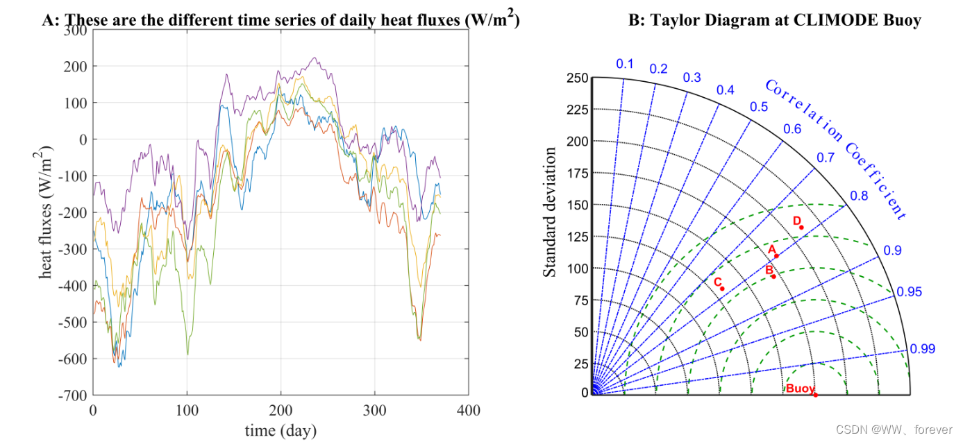
MATLAB代码如下：

clear
%% 导入数据
pathFigure= '.\Figures\' ;
load taylordiag_egdata.mat

% Get statistics from time series:
for ii = 2:size(BUOY,1)
    C = allstats(BUOY(1,:),BUOY(ii,:));
    statm(ii,:) = C(:,2);
end
statm(1,:) = C(:,1);

% Plot:
figureUnits = 'centimeters';
figureWidth = 30; 
figureHeight = 12;

figure(1)
set(gcf, 'Units', figureUnits, 'Position', [0 0 figureWidth figureHeight]);
ax = ptable([2 3],[2 2;4 6]);
iw=1;
jw=2;
alphab = 'ABCDEFG';

subplot(iw,jw,1); 
plot(BUOY');
grid on;
xlabel('time (day)','FontSize',12,'FontName','Times New Roman');
ylabel('heat fluxes (W/m^2)','FontSize',12,'FontName','Times New Roman');
title(sprintf('%s: These are the different time series of daily heat fluxes (W/m^2)','A'),'fontweight','bold','FontSize',12,'FontName','Times New Roman');
set(gca,'FontSize',12,'Fontname', 'Times New Roman');
set(gca,'Layer','top');

subplot(iw,jw,2); 
hold on
[pp tt axl] = taylordiag(squeeze(statm(:,2)),squeeze(statm(:,3)),squeeze(statm(:,4)),...
            'tickRMS',[25:25:150],'titleRMS',0,'tickRMSangle',135,'showlabelsRMS',0,'widthRMS',1,...
            'tickSTD',[25:25:250],'limSTD',250,...
            'tickCOR',[.1:.1:.9 .95 .99],'showlabelsCOR',1,'titleCOR',1);

for ii = 1 : length(tt)
    set(tt(ii),'fontsize',9,'fontweight','bold')
    set(pp(ii),'markersize',12)
    if ii == 1
        set(tt(ii),'String','Buoy');
    else
        set(tt(ii),'String',alphab(ii-1));
    end
end
title(sprintf('%s: Taylor Diagram at CLIMODE Buoy','B'),'fontweight','bold','FontSize',12,'FontName','Times New Roman');

tt = axl(2).handle;
for ii = 1 : length(tt)
    set(tt(ii),'fontsize',10,'fontweight','normal','FontSize',12,'FontName','Times New Roman');
end
set(axl(1).handle,'fontweight','normal','FontSize',12,'FontName','Times New Roman');
set(gca,'FontSize',12,'Fontname', 'Times New Roman');
set(gca,'Layer','top');

str= strcat(pathFigure, "Fig.1", '.tiff');
print(gcf, '-dtiff', '-r600', str);