时间序列是指在一段时间内发生的任何可量化的度量或事件。尽管这听起来微不足道，但几乎任何东西都可以被认为是时间序列。一个月里你每小时的平均心率，一年里一只股票的日收盘价，一年里某个城市每周发生的交通事故数。

在任何一段时间段内记录这些信息都被认为是一个时间序列。对于这些例子中的每一个，都有事件发生的频率(每天、每周、每小时等)和事件发生的时间长度(一个月、一年、一天等)。

在本教程中，我们将使用 PyTorch-LSTM 进行深度学习时间序列预测。

我们的目标是接收一个值序列，预测该序列中的下一个值。最简单的方法是使用自回归模型，我们将专注于使用LSTM来解决这个问题。

数据准备

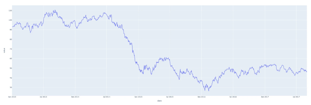
让我们看一个时间序列样本。下图显示了2013年至2018年石油价格的一些数据。

’

技术提升

技术要学会分享、交流，不建议闭门造车。一个人走的很快、一堆人可以走的更远。

完整代码、数据、技术交流提升， 均可加交流群获取，群友已超过2000人，添加时切记的备注方式为：来源+兴趣方向，方便找到志同道合的朋友。

方式①、添加微信号：pythoner666，备注：来自 CSDN + python
方式②、微信搜索公众号：Python学习与数据挖掘，后台回复：加群

这只是一个日期轴上单个数字序列的图。下表显示了这个时间序列的前10个条目。每天都有价格数据。

 date       dcoilwtico  
 2013-01-01 NaN  
 2013-01-02 93.14  
 2013-01-03 92.97  
 2013-01-04 93.12  
 2013-01-07 93.20  
 2013-01-08 93.21  
 2013-01-09 93.08  
 2013-01-10 93.81  
 2013-01-11 93.60  
 2013-01-14 94.27

许多机器学习模型在标准化数据上的表现要好得多。标准化数据的标准方法是对数据进行转换，使得每一列的均值为0，标准差为1。下面的代码scikit-learn进行标准化

 from sklearn.preprocessing import StandardScaler  
   
 # Fit scalers  
 scalers = {}  
 for x in df.columns:  
   scalers[x] = StandardScaler().fit(df[x].values.reshape(-1, 1))  
   
 # Transform data via scalers  
 norm_df = df.copy()  
 for i, key in enumerate(scalers.keys()):  
   norm = scalers[key].transform(norm_df.iloc[:, i].values.reshape(-1, 1))  
   norm_df.iloc[:, i] = norm

我们还希望数据具有统一的频率——在这个例子中，有这5年里每天的石油价格，如果你的数据情况并非如此，Pandas有几种不同的方法来重新采样数据以适应统一的频率，请参考我们公众号以前的文章

对于训练数据我们需要将完整的时间序列数据截取成固定长度的序列。假设我们有一个序列：[1, 2, 3, 4, 5, 6]。

通过选择长度为 3 的序列，我们可以生成以下序列及其相关目标：

[Sequence] Target

[1, 2, 3] → 4

[2, 3, 4] → 5

[3, 4, 5] → 6

或者说我们定义了为了预测下一个值需要回溯多少步。我们将这个值称为训练窗口，而要预测的值的数量称为预测窗口。在这个例子中，它们分别是3和1。下面的函数详细说明了这是如何完成的。

 # 如上所示，定义一个创建序列和目标的函数  
 def generate_sequences(df: pd.DataFrame, tw: int, pw: int, target_columns, drop_targets=False):  
   '''  
  df: Pandas DataFrame of the univariate time-series  
  tw: Training Window - Integer defining how many steps to look back  
  pw: Prediction Window - Integer defining how many steps forward to predict  
   
  returns: dictionary of sequences and targets for all sequences  
  '''  
   data = dict() # Store results into a dictionary  
   L = len(df)  
   for i in range(L-tw):  
     # Option to drop target from dataframe  
     if drop_targets:  
       df.drop(target_columns, axis=1, inplace=True)  
   
     # Get current sequence    
     sequence = df[i:i+tw].values  
     # Get values right after the current sequence  
     target = df[i+tw:i+tw+pw][target_columns].values  
     data[i] = {'sequence': sequence, 'target': target}  
   return data

这样我们就可以在PyTorch中使用Dataset类自定义数据集

 class SequenceDataset(Dataset):  
   
   def __init__(self, df):  
     self.data = df  
   
   def __getitem__(self, idx):  
     sample = self.data[idx]  
     return torch.Tensor(sample['sequence']), torch.Tensor(sample['target'])  
     
   def __len__(self):  
     return len(self.data)

然后，我们可以使用PyTorch DataLoader来遍历数据。使用DataLoader的好处是它在内部自动进行批处理和数据的打乱，所以我们不必自己实现它，代码如下:

 # 这里我们为我们的模型定义属性  
   
 BATCH_SIZE = 16 # Training batch size  
 split = 0.8 # Train/Test Split ratio  
   
 sequences = generate_sequences(norm_df.dcoilwtico.to_frame(), sequence_len, nout, 'dcoilwtico')  
 dataset = SequenceDataset(sequences)  
   
 # 根据拆分比例拆分数据，并将每个子集加载到单独的DataLoader对象中  
 train_len = int(len(dataset)*split)  
 lens = [train_len, len(dataset)-train_len]  
 train_ds, test_ds = random_split(dataset, lens)  
 trainloader = DataLoader(train_ds, batch_size=BATCH_SIZE, shuffle=True, drop_last=True)  
 testloader = DataLoader(test_ds, batch_size=BATCH_SIZE, shuffle=True, drop_last=True)

在每次迭代中，DataLoader将产生16个(批量大小)序列及其相关目标，我们将这些目标传递到模型中。

模型架构

我们将使用一个单独的LSTM层，然后是模型的回归部分的一些线性层，当然在它们之间还有dropout层。该模型将为每个训练输入输出单个值。

 class LSTMForecaster(nn.Module):  
  
   def __init__(self, n_features, n_hidden, n_outputs, sequence_len, n_lstm_layers=1, n_deep_layers=10, use_cuda=False, dropout=0.2):  
     '''  
    n_features: number of input features (1 for univariate forecasting)  
    n_hidden: number of neurons in each hidden layer  
    n_outputs: number of outputs to predict for each training example  
    n_deep_layers: number of hidden dense layers after the lstm layer  
    sequence_len: number of steps to look back at for prediction  
    dropout: float (0 < dropout < 1) dropout ratio between dense layers  
    '''  
     super().__init__()  
   
     self.n_lstm_layers = n_lstm_layers  
     self.nhid = n_hidden  
     self.use_cuda = use_cuda # set option for device selection  
   
     # LSTM Layer  
     self.lstm = nn.LSTM(n_features,  
                         n_hidden,  
                         num_layers=n_lstm_layers,  
                         batch_first=True) # As we have transformed our data in this way  
       
     # first dense after lstm  
     self.fc1 = nn.Linear(n_hidden * sequence_len, n_hidden)  
     # Dropout layer  
     self.dropout = nn.Dropout(p=dropout)  
   
     # Create fully connected layers (n_hidden x n_deep_layers)  
     dnn_layers = []  
     for i in range(n_deep_layers):  
       # Last layer (n_hidden x n_outputs)  
       if i == n_deep_layers - 1:  
         dnn_layers.append(nn.ReLU())  
         dnn_layers.append(nn.Linear(nhid, n_outputs))  
       # All other layers (n_hidden x n_hidden) with dropout option  
       else:  
         dnn_layers.append(nn.ReLU())  
         dnn_layers.append(nn.Linear(nhid, nhid))  
         if dropout:  
           dnn_layers.append(nn.Dropout(p=dropout))  
     # compile DNN layers  
     self.dnn = nn.Sequential(*dnn_layers)  
   
   def forward(self, x):  
   
     # Initialize hidden state  
     hidden_state = torch.zeros(self.n_lstm_layers, x.shape[0], self.nhid)  
     cell_state = torch.zeros(self.n_lstm_layers, x.shape[0], self.nhid)  
   
     # move hidden state to device  
     if self.use_cuda:  
       hidden_state = hidden_state.to(device)  
       cell_state = cell_state.to(device)  
           
     self.hidden = (hidden_state, cell_state)  
   
     # Forward Pass  
     x, h = self.lstm(x, self.hidden) # LSTM  
     x = self.dropout(x.contiguous().view(x.shape[0], -1)) # Flatten lstm out  
     x = self.fc1(x) # First Dense  
     return self.dnn(x) # Pass forward through fully connected DNN.

我们设置了2个可以自由地调优的参数n_hidden和n_deep_players。更大的参数意味着模型更复杂和更长的训练时间，所以这里我们可以使用这两个参数灵活调整。

剩下的参数如下：sequence_len指的是训练窗口，nout定义了要预测多少步;将sequence_len设置为180,nout设置为1，意味着模型将查看180天(半年)后的情况，以预测明天将发生什么。

 nhid = 50 # Number of nodes in the hidden layer  
 n_dnn_layers = 5 # Number of hidden fully connected layers  
 nout = 1 # Prediction Window  
 sequence_len = 180 # Training Window  
   
 # Number of features (since this is a univariate timeseries we'll set  
 # this to 1 -- multivariate analysis is coming in the future)  
 ninp = 1  
   
 # Device selection (CPU | GPU)  
 USE_CUDA = torch.cuda.is_available()  
 device = 'cuda' if USE_CUDA else 'cpu'  
   
 # Initialize the model  
 model = LSTMForecaster(ninp, nhid, nout, sequence_len, n_deep_layers=n_dnn_layers, use_cuda=USE_CUDA).to(device)

模型训练

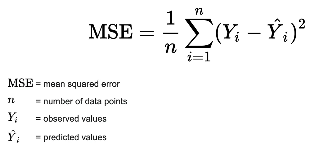
定义好模型后，我们可以选择损失函数和优化器，设置学习率和周期数，并开始我们的训练循环。由于这是一个回归问题(即我们试图预测一个连续值)，最简单也是最安全的损失函数是均方误差。这提供了一种稳健的方法来计算实际值和模型预测值之间的误差。

优化器和损失函数如下：

 # Set learning rate and number of epochs to train over  
 lr = 4e-4  
 n_epochs = 20  
   
 # Initialize the loss function and optimizer  
 criterion = nn.MSELoss().to(device)  
 optimizer = torch.optim.AdamW(model.parameters(), lr=lr)

下面就是训练循环的代码：在每次训练迭代中，我们将计算之前创建的训练集和验证集的损失:

# Lists to store training and validation losses  
t_losses, v_losses = [], []  
# Loop over epochs  
for epoch in range(n_epochs):  
  train_loss, valid_loss = 0.0, 0.0  
  
  # train step  
  model.train()  
  # Loop over train dataset  
  for x, y in trainloader:  
    optimizer.zero_grad()  
    # move inputs to device  
    x = x.to(device)  
    y  = y.squeeze().to(device)  
    # Forward Pass  
    preds = model(x).squeeze()  
    loss = criterion(preds, y) # compute batch loss  
    train_loss += loss.item()  
    loss.backward()  
    optimizer.step()  
  epoch_loss = train_loss / len(trainloader)  
  t_losses.append(epoch_loss)  
    
  # validation step  
  model.eval()  
  # Loop over validation dataset  
  for x, y in testloader:  
    with torch.no_grad():  
      x, y = x.to(device), y.squeeze().to(device)  
      preds = model(x).squeeze()  
      error = criterion(preds, y)  
    valid_loss += error.item()  
  valid_loss = valid_loss / len(testloader)  
  v_losses.append(valid_loss)  
        
  print(f'{epoch} - train: {epoch_loss}, valid: {valid_loss}')  
plot_losses(t_losses, v_losses)  

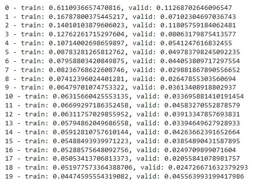
这样模型已经训练好了，可以评估预测了。

推理

我们调用训练过的模型来预测未打乱的数据，并比较预测与真实观察有多大不同。

def make_predictions_from_dataloader(model, unshuffled_dataloader):  
  model.eval()  
  predictions, actuals = [], []  
  for x, y in unshuffled_dataloader:  
    with torch.no_grad():  
      p = model(x)  
      predictions.append(p)  
      actuals.append(y.squeeze())  
  predictions = torch.cat(predictions).numpy()  
  actuals = torch.cat(actuals).numpy()  
  return predictions.squeeze(), actuals  

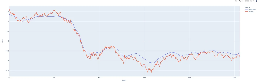
石油历史上的常态化预测与实际价格

我们的预测看起来还不错!预测的效果还可以，表明我们没有过度拟合模型，让我们看看能否用它来预测未来。

预测

如果我们将历史定义为预测时刻之前的序列，算法很简单:

1. 从历史(训练窗口长度)中获取最新的有效序列。

2. 将最新的序列输入模型并预测下一个值。

3. 将预测值附加到历史记录上。

4. 迭代重复步骤1。

这里需要注意的是，根据训练模型时选择的参数，你预测的越长（远），模型就越容易表现出它自己的偏差，开始预测平均值。因此，如果没有必要，我们不希望总是预测得太超前，因为这会影响预测的准确性。

这在下面的函数中实现:

def one_step_forecast(model, history):  
      '''  
      model: PyTorch model object  
      history: a sequence of values representing the latest values of the time   
      series, requirement -> len(history.shape) == 2  
      
      outputs a single value which is the prediction of the next value in the  
      sequence.  
      '''  
      model.cpu()  
      model.eval()  
      with torch.no_grad():  
        pre = torch.Tensor(history).unsqueeze(0)  
        pred = self.model(pre)  
      return pred.detach().numpy().reshape(-1)  
  
  def n_step_forecast(data: pd.DataFrame, target: str, tw: int, n: int, forecast_from: int=None, plot=False):  
      '''  
      n: integer defining how many steps to forecast  
      forecast_from: integer defining which index to forecast from. None if  
      you want to forecast from the end.  
      plot: True if you want to output a plot of the forecast, False if not.  
      '''  
      history = data[target].copy().to_frame()  
        
      # Create initial sequence input based on where in the series to forecast   
      # from.  
      if forecast_from:  
        pre = list(history[forecast_from - tw : forecast_from][target].values)  
      else:  
        pre = list(history[self.target])[-tw:]  
  
      # Call one_step_forecast n times and append prediction to history  
      for i, step in enumerate(range(n)):  
        pre_ = np.array(pre[-tw:]).reshape(-1, 1)  
        forecast = self.one_step_forecast(pre_).squeeze()  
        pre.append(forecast)  
        
      # The rest of this is just to add the forecast to the correct time of   
      # the history series  
      res = history.copy()  
      ls = [np.nan for i in range(len(history))]  
  
      # Note: I have not handled the edge case where the start index + n is   
      # before the end of the dataset and crosses past it.  
      if forecast_from:  
        ls[forecast_from : forecast_from + n] = list(np.array(pre[-n:]))  
        res['forecast'] = ls  
        res.columns = ['actual', 'forecast']  
      else:  
        fc = ls + list(np.array(pre[-n:]))  
        ls = ls + [np.nan for i in range(len(pre[-n:]))]  
        ls[:len(history)] = history[self.target].values  
        res = pd.DataFrame([ls, fc], index=['actual', 'forecast']).T  
      return res  

我们来看看实际的效果

我们在这个时间序列的中间从不同的地方进行预测，这样我们就可以将预测与实际发生的情况进行比较。我们的预测程序，可以从任何地方对任何合理数量的步骤进行预测，红线表示预测。（这些图表显示的是y轴上的标准化后的价格）

预测2013年第三季度后200天

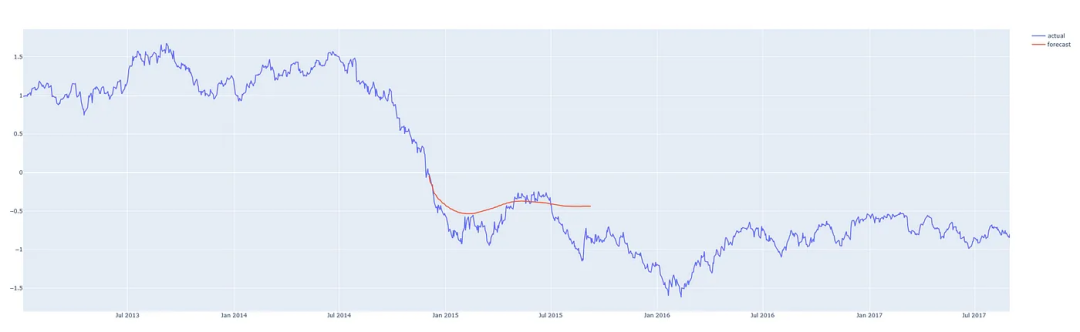
预测2014/15 后200天

从2016年第一季度开始预测200天

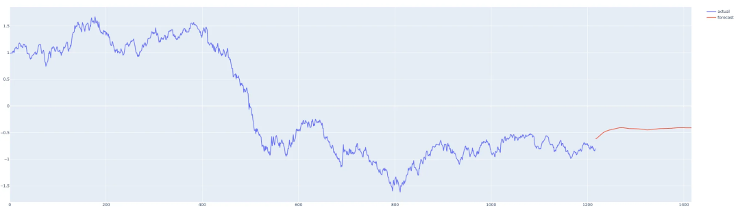
从数据的最后一天开始预测200天

总结

我们这个模型表现的还算一般!但是我们通过这个示例完整的介绍了时间序列预测的全部过程，我们可以通过尝试架构和参数的调整使模型变得得更好，预测得更准确。

本文只处理单变量时间序列，其中只有一个值序列。还有一些方法可以使用多个系列来进行预测。这被称为多元时间序列预测，我将在以后的文章中介绍。