Transformer 之 各种 Attention 原理和实现

本文将介绍Transformer 中常见的Attention的原理和实现，其中包括： Self Attention、Spatial Attention、Temporal Attention、Cross Attention、Grouped Attention、Tensor Product Attention、FlashAttention。通过深入理解这些 Attention 机制，开发者可以根据具体任务需求选择最合适的架构，从而在模型性能、效率和内存占用之间找到最佳平衡。

---

文章目录

• Transformer 之 各种 Attention 原理和实现
• • @[toc]
  • 1. Self-Attention
  • • 1.1 基础原理
    • 1.2 代码
    • 1.3 多头扩展（多头注意力， MHA）
    • 1.4 MHA 代码
    • 1.5 优势与局限
  • 2. Spatial Attention：视觉任务的空间聚焦
  • • 2.1 结构设计
    • 2.2 代码
  • 3. Temporal Attention
  • • 3.1 原理
    • 3.2 代码
  • 4. Cross-Attention：跨模态交互的桥梁
  • • 4.1 交互机制
    • 4.4 代码
  • 5. Grouped-Query Attention
  • • 5.1 原理
    • 5.2 代码
  • 6. Tensor Product Attention
  • • 6.1 原理
    • 6.2 代码
  • 7. FlashAttention
  • • 7.1 原理
  • 8 对比
  • 9 测试代码
  • 引用

1. Self-Attention

1.1 基础原理

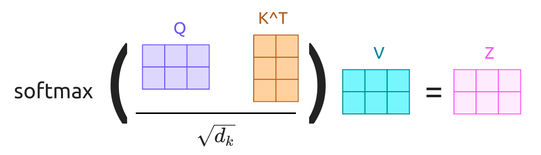
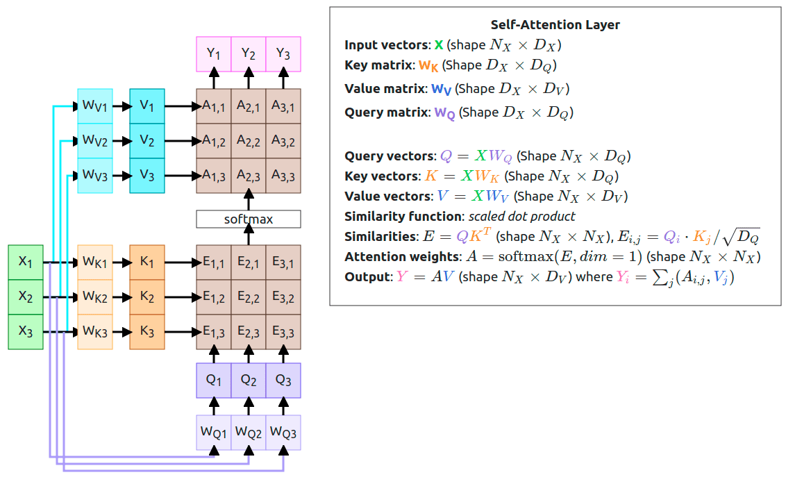
2017年，论文《Transformer ：Attention Is All You Need》提出，Self-Attention（自注意力）是 Transformer 模型的核心组件，其核心思想是让每个位置的词向量同时关注序列中所有其他位置的信息，从而捕捉全局依赖关系。其计算过程分为以下步骤：

1. 线性投影：将输入序列 $X\in {\mathbb{R}}^{n\times d}$ 分别映射为查询（Query）、键（Key）和值（Value）矩阵：
   $$Q=X{W}^Q,K=X{W}^K,V=X{W}^V$$
   其中 $W^Q,W^K,W^V\in {\mathbb{R}}^{d\times d_k}$ 是可学习的权重矩阵。

2. 注意力分数计算：计算查询与键的点积相似度，并通过缩放因子 $\sqrt{d_k}$ 防止梯度消失：
   $$\text{scores}=\frac{Q{K}^T}{\sqrt{d_k}}$$

3. 归一化与加权求和：使用 Softmax 对分数进行归一化得到注意力权重 $\alpha$，并与值矩阵相乘得到输出：
   $$\text{Attention}(Q,K,V)=\text{Softmax}(\text{scores})\cdot V$$

其具体计算过程如下图所示：

1.2 代码

import torch
import torch.nn as nn
import torch.nn.functional as F

class SelfAttention(nn.Module):
    def __init__(self, input_dim, d_k):
        super(SelfAttention, self).__init__()
        self.W_q = nn.Linear(input_dim, d_k)
        self.W_k = nn.Linear(input_dim, d_k)
        self.W_v = nn.Linear(input_dim, d_k)

    def forward(self, x):
        Q = self.W_q(x)
        K = self.W_k(x)
        V = self.W_v(x)
        scores = torch.matmul(Q, K.transpose(-2, -1)) / torch.sqrt(torch.tensor(Q.size(-1)).float())
        attn_weights = F.softmax(scores, dim=-1)
        output = torch.matmul(attn_weights, V)
        return output

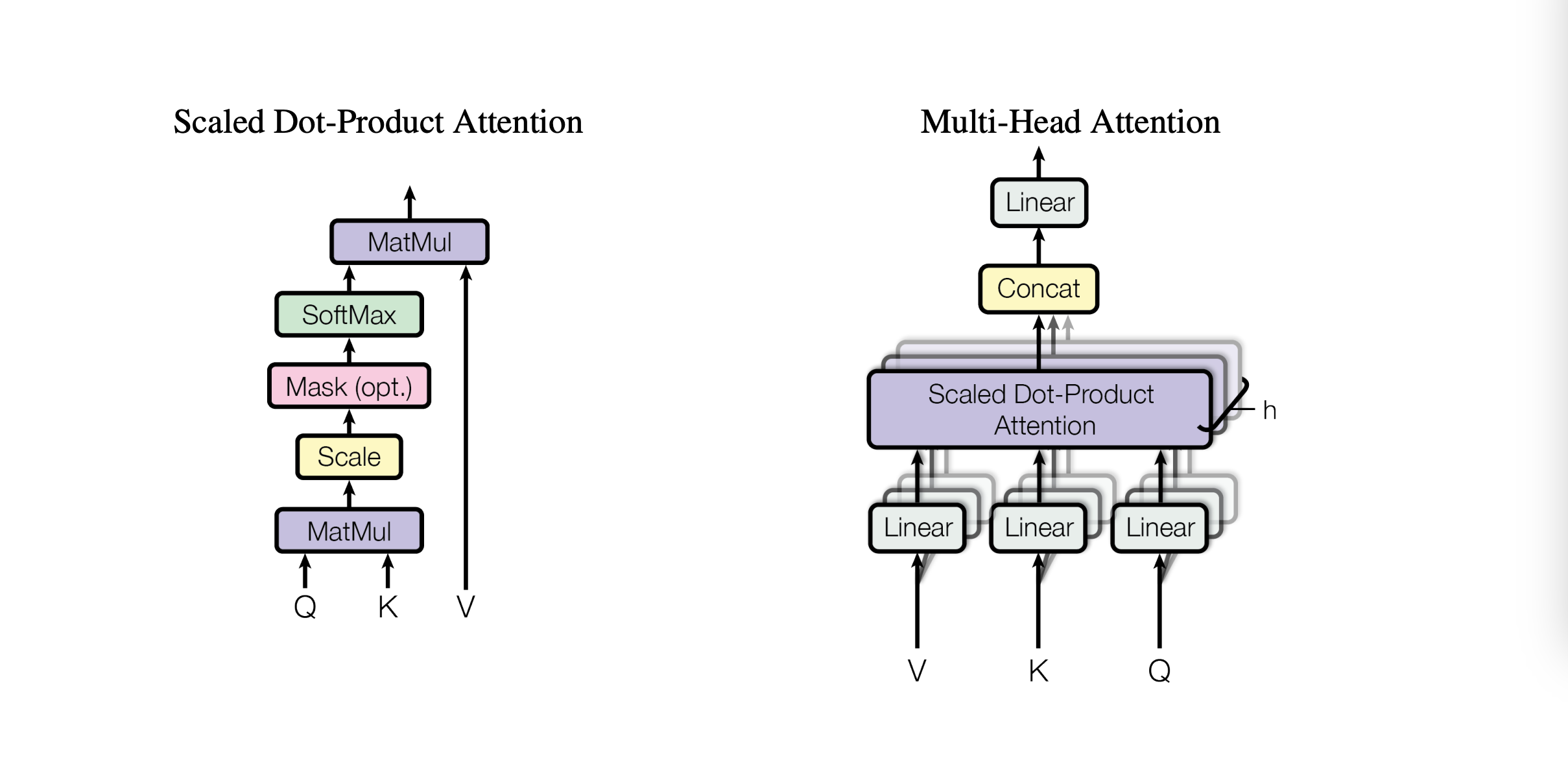
1.3 多头扩展（多头注意力， MHA）

为了捕捉不同子空间的语义信息，Transformer 引入了多头注意力（Multi-Head Attention）。将查询、键、值矩阵拆分为 $h$ 个独立的头，每个头独立计算注意力，最后将结果拼接并投影回原始维度：
$$\text{MultiHead}(Q,K,V)=\text{Concat}({\text{head}}_1,\dots ,{\text{head}}_h)W^O$$
其中 ${\text{head}}_i=\text{Attention}(Q{W}_i^Q,K{W}_i^K,V{W}_i^V)$。

下图左边表示Self-Attention的结构，右边为MHA的结构，可以看出MHA是在 Self-Attention的基础上，分出了很多个独立头。

1.4 MHA 代码

class MultiHeadAttention(nn.Module):
    def __init__(self, input_dim, num_heads, d_k):
        super(MultiHeadAttention, self).__init__()
        self.input_dim = input_dim
        self.num_heads = num_heads
        self.d_k = d_k
        self.head_dim = d_k // num_heads

        # 线性层用于生成 Q, K, V
        self.W_q = nn.Linear(input_dim, d_k)
        self.W_k = nn.Linear(input_dim, d_k)
        self.W_v = nn.Linear(input_dim, d_k)
        self.W_o = nn.Linear(d_k, input_dim)

    def forward(self, x):
        batch_size, seq_len, _ = x.size()

        # 生成 Q, K, V
        Q = self.W_q(x).view(batch_size, seq_len, self.num_heads, self.head_dim).transpose(1, 2)
        K = self.W_k(x).view(batch_size, seq_len, self.num_heads, self.head_dim).transpose(1, 2)
        V = self.W_v(x).view(batch_size, seq_len, self.num_heads, self.head_dim).transpose(1, 2)

        # 计算注意力分数
        scores = torch.matmul(Q, K.transpose(-2, -1)) / torch.sqrt(torch.tensor(self.head_dim).float())
        attn_weights = F.softmax(scores, dim=-1)

        # 计算加权和
        output = torch.matmul(attn_weights, V)
        output = output.transpose(1, 2).contiguous().view(batch_size, seq_len, -1)

        # 输出投影
        output = self.W_o(output)
        return output

1.5 优势与局限

• 优势：并行计算能力强，能有效捕捉长距离依赖。
• 局限：时间复杂度为 $O(n^2)$，处理超长序列时内存占用高。

---

2. Spatial Attention：视觉任务的空间聚焦

2.1 结构设计

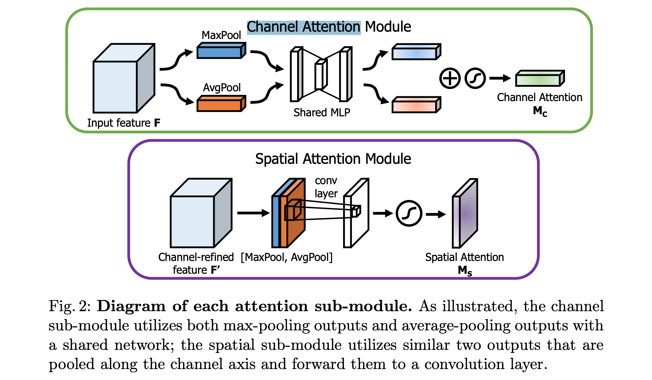
2018年，论文《CBAM: Convolutional Block Attention Module》提出，Spatial Attention（空间注意力） 和 Channel Attention（通道注意力）。他们主要用于计算机视觉任务，其目标是通过学习空间位置的重要性权重，增强关键区域的特征表示。典型Spatial Attention（空间注意力）实现步骤如下：

1. 特征压缩：将输入特征图 $X\in {\mathbb{R}}^{C\times H\times W}$ 沿通道维度压缩，得到空间特征：
   $$f=\text{MaxPool}(X)+\text{AvgPool}(X)$$

2. 权重生成：通过卷积层生成空间注意力图 $M\in {\mathbb{R}}^{1\times H\times W}$：
   $$M=\sigma (\text{Conv}(f))$$
   其中 $\sigma$ 为 Sigmoid 激活函数。

3. 特征增强：将注意力图与原始特征图逐元素相乘：
   $$X^{\prime }=X\odot M$$

下图对应论文中 Spatial Attention（空间注意力） 和 Channel Attention（通道注意力） 的结构：

下图表示CBAM结构：

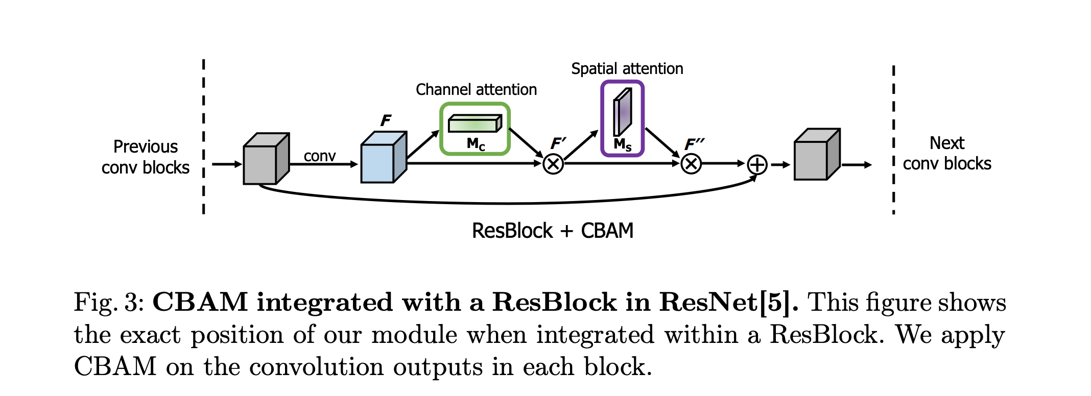
因此，其应用场景主要包括三个领域：图像分类：聚焦目标物体区域、目标检测：增强边界框特征、语义分割：细化区域边界。 在Swin Transformer中，也使用了Spatial Attention（空间注意力）通过窗口划分实现局部空间注意力。

2.2 代码

class SpatialAttention(nn.Module):
    def __init__(self, kernel_size=7):
        super(SpatialAttention, self).__init__()
        assert kernel_size in (3, 7), 'kernel size must be 3 or 7'
        padding = 3 if kernel_size == 7 else 1
        self.conv1 = nn.Conv2d(2, 1, kernel_size, padding=padding, bias=False)
        self.sigmoid = nn.Sigmoid()

    def forward(self, x):
        avg_out = torch.mean(x, dim=1, keepdim=True)
        max_out, _ = torch.max(x, dim=1, keepdim=True)
        x = torch.cat([avg_out, max_out], dim=1)
        x = self.conv1(x)
        return self.sigmoid(x)

---

3. Temporal Attention

3.1 原理

根论文《Temporal Attention for Language Models》，Temporal Attention（时间感知自注意力）是对Transformer自注意力机制的扩展，通过引入时间矩阵将时间信息融入注意力权重计算，使模型能够生成时间特定的上下文词表示。

1. 核心思想

• 在标准自注意力的基础上，引入时间矩阵 $T$，该矩阵编码了文本序列对应的时间点信息。
• 时间矩阵与查询矩阵 $Q$ 和键矩阵 $K$ 相乘，使注意力权重依赖于时间，公式为：
  $$\text{TemporalAttention}(Q,K,V,T)=\text{softmax}\left(\frac{Q\cdot (T^{\top }T/\Vert T\Vert )\cdot K^{\top }}{\sqrt{d_k}}\right)\cdot V$$
  其中 $T$ 由时间点嵌入矩阵通过线性变换得到，用于缩放注意力分数，使模型在计算词间依赖时考虑时间因素。

2. 输入与输出

• 输入：文本序列嵌入 $X\in {\mathbb{R}}^{n\times D}$ 和时间点 $t$。
• 时间嵌入：将时间点 $t$ 映射为 $D$ 维向量，生成时间嵌入矩阵 $X^t$，其中每个时间点对应一个嵌入向量。
• 线性变换：通过可学习矩阵 $W_T$ 将时间嵌入转换为 $T\in {\mathbb{R}}^{n\times d_k}$，与 $Q,K,V$ 维度一致。

3. 与自注意力的区别

• 时间整合方式：自注意力仅建模词间依赖，而Temporal Attention通过时间矩阵将时间作为条件，使注意力权重具有时间敏感性。
• 输入扩展：无需修改输入文本（如添加时间令牌），而是通过模型内部机制整合时间信息。

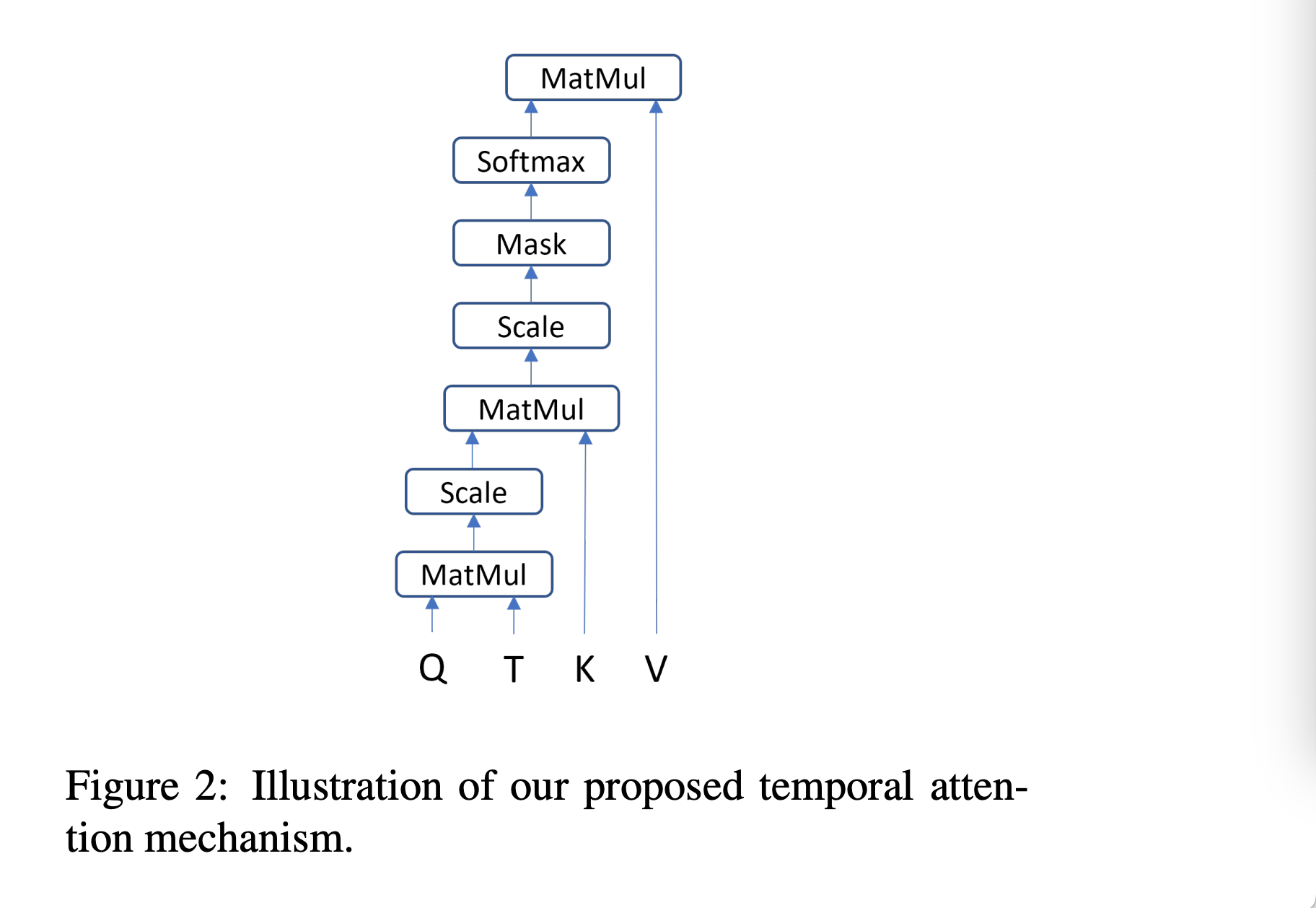
其实就是增加了一个T变量，只对应时间维度，重点强化时间维度的重要性。如下图所示，展示了 Temporal Attention 的网络结构。

3.2 代码

class TemporalAttention(nn.Module):
    def __init__(self, input_dim, d_k, time_emb_dim):
        super(TemporalAttention, self).__init__()
        self.input_dim = input_dim  # 输入文本嵌入维度
        self.d_k = d_k  # Q/K/V维度
        self.time_emb_dim = time_emb_dim  # 时间嵌入维度
        
        # 文本的Q/K/V线性层
        self.W_q = nn.Linear(input_dim, d_k)
        self.W_k = nn.Linear(input_dim, d_k)
        self.W_v = nn.Linear(input_dim, d_k)
        
        # 时间嵌入的线性层（将时间点映射到d_k维度）
        self.W_t = nn.Linear(time_emb_dim, d_k)
    
    def forward(self, x, time_points):
        batch_size, seq_len, _ = x.size()
        num_time_points = time_points.size(1)  # 假设每个序列对应一个时间点
        
        # 生成文本的Q/K/V
        Q = self.W_q(x)  # (batch_size, seq_len, d_k)
        K = self.W_k(x)  # (batch_size, seq_len, d_k)
        V = self.W_v(x)  # (batch_size, seq_len, d_k)
        
        # 生成时间矩阵T：将时间点嵌入扩展为序列长度一致的矩阵
        time_emb = self.W_t(time_points)  # (batch_size, 1, d_k)
        T = time_emb.repeat(1, seq_len, 1)  # (batch_size, seq_len, d_k)
        
        # 计算时间矩阵的全局范数（Frobenius范数）
        T_norm = torch.norm(T, p='fro', dim=(1, 2), keepdim=True)  # (batch_size, 1, 1)
        T_scaled = (T.transpose(1, 2) @ T) / (T_norm + 1e-8)  # (batch_size, d_k, d_k)
                                                             # a @ b 就相当于 torch.matmul(a, b)
        
        # 计算注意力分数：Q * T_scaled * K^T
        scores = torch.matmul(Q, T_scaled)  # (batch_size, seq_len, d_k)
        scores = torch.matmul(scores, K.transpose(1, 2))  # (batch_size, seq_len, seq_len)
        scores = scores / torch.sqrt(torch.tensor(self.d_k, dtype=torch.float32))
        
        # 归一化和加权求和
        attn_weights = F.softmax(scores, dim=-1)
        output = torch.matmul(attn_weights, V)
        return output, attn_weights

代码解释：

1. 初始化：

   • W_q, W_k, W_v 处理文本嵌入生成Q/K/V。
   • W_t 将时间点嵌入（如时间戳）映射到与Q/K/V同维度的矩阵 $T$。 (这里是相较于self-attention增加的部分)

2. 时间矩阵生成：

   • 假设每个序列对应一个时间点，将时间嵌入重复为序列长度，生成 $T\in {\mathbb{R}}^{batch\times seq\times d_k}$。
   • 通过 $T^{\top }T/\Vert T\Vert$ 计算时间缩放因子，确保维度匹配并避免数值不稳定。

3. 注意力计算：

   • 分数计算时引入时间缩放因子，使注意力权重依赖于时间点 $t$。
   • 输出为加权后的Value矩阵，携带时间特定的上下文信息。

4. 测试实例：

   • 输入包含文本嵌入和时间点嵌入，验证输出形状符合预期，确保时间信息正确融入注意力机制。

该实现，确保时间信息在注意力计算中的显式建模，适用于需要时间感知的NLP任务（如语义变化检测、时序问答等）和视频任务（如理解和生成）。

下图展示了 Temporal Attention 的简化网络结构：

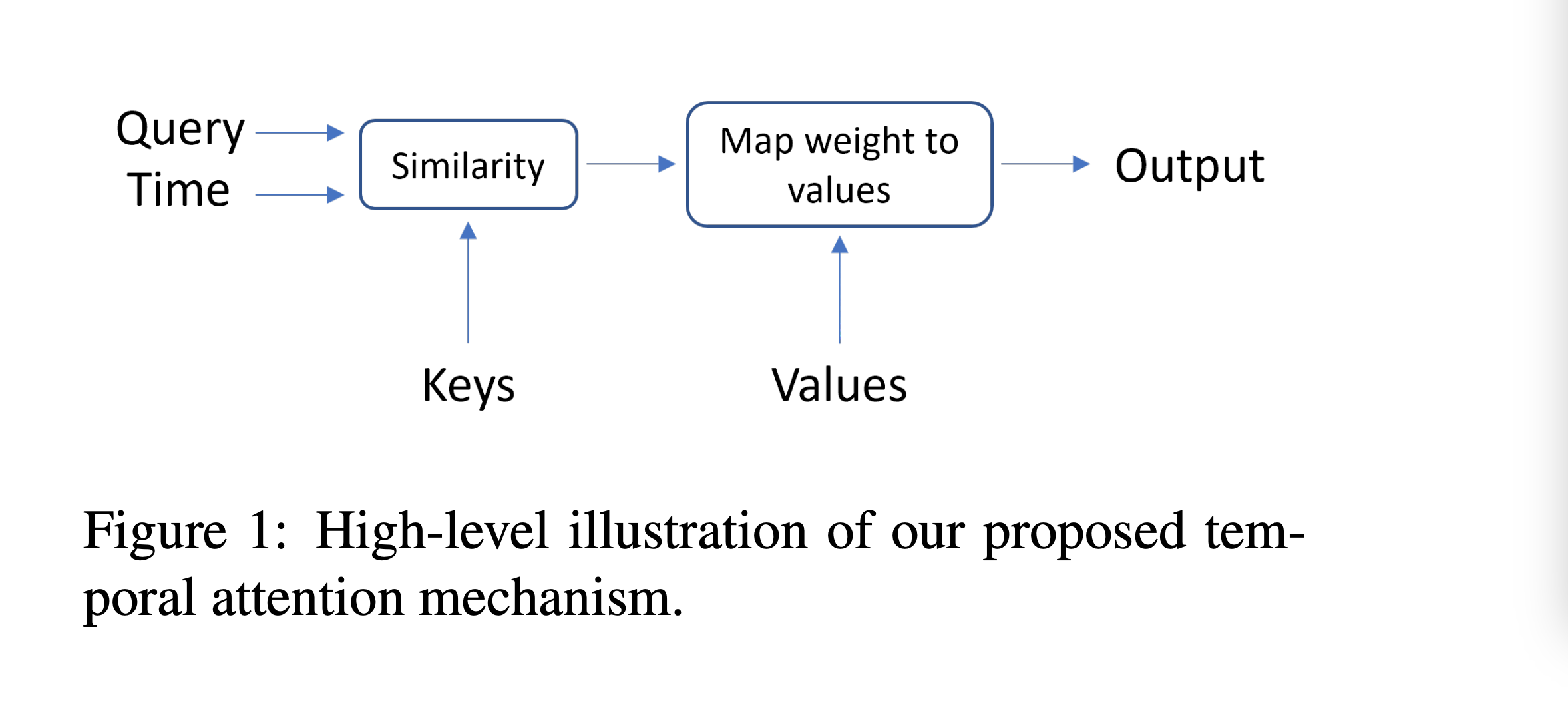
基于上面的原理和实现，Temporal Attention存在一些优势。首先是，时间感知建模：通过时间矩阵直接影响注意力权重，无需修改输入文本，保持模型通用性。 其次是，跨时间泛化：适用于文本和视频的语义变化检测等任务，生成不同时间点的差异化表示，提升时序相关任务性能。 最后是，轻量化扩展：仅增加时间线性层，内存开销可忽略，优于输入级时间令牌拼接方法。

---

4. Cross-Attention：跨模态交互的桥梁

4.1 交互机制

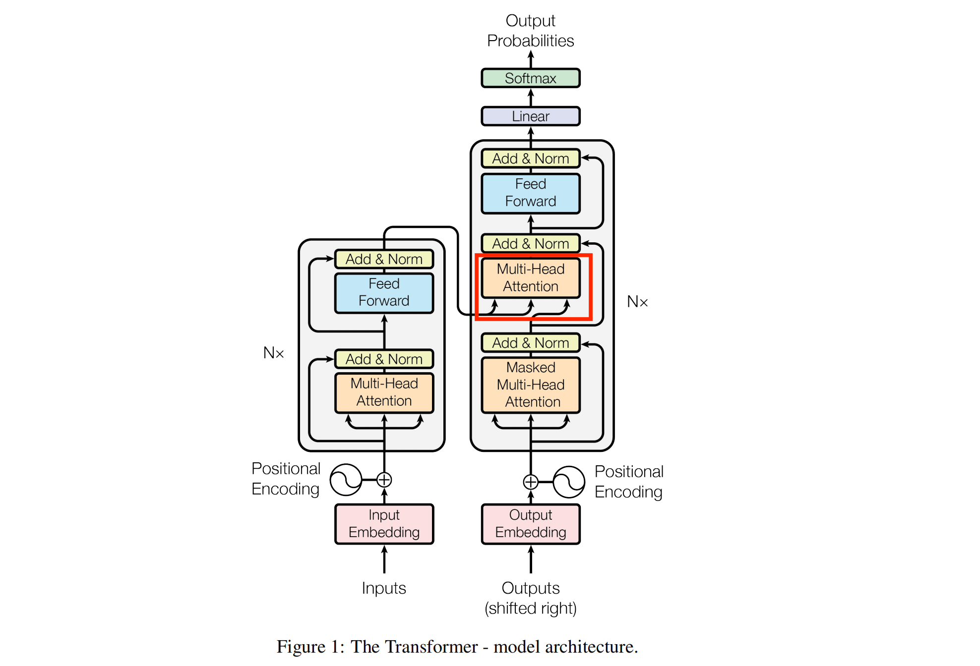
2017年，论文《Transformer ：Attention Is All You Need》除了提出，Self-Attention（自注意力）之外，还提出了Cross-Attention（交叉注意力），用于处理两个不同序列之间的交互，例如机器翻译中的源语言与目标语言。如下图所示：

其计算流程如下：

1. 投影操作：
   $$Q=\text{Decoder\_Output}\cdot W^Q,K=\text{Encoder\_Output}\cdot W^K,V=\text{Encoder\_Output}\cdot W^V$$

2. 注意力计算：
   $$\text{CrossAttention}(Q,K,V)=\text{Softmax}\left(\frac{Q{K}^T}{\sqrt{d_k}}\right)\cdot V$$

其应用场景非常多，比如：机器翻译：解码器关注编码器的输出，图像字幕生成：语言模型关注图像特征，特别是多模态融合：文本与视觉特征的交互。

4.4 代码

class CrossAttention(nn.Module):
    def __init__(self, input_dim, d_k):
        super(CrossAttention, self).__init__()
        self.W_q = nn.Linear(input_dim, d_k)
        self.W_k = nn.Linear(input_dim, d_k)
        self.W_v = nn.Linear(input_dim, d_k)

    def forward(self, x1, x2):
        Q = self.W_q(x1)
        K = self.W_k(x2)
        V = self.W_v(x2)
        scores = torch.matmul(Q, K.transpose(-2, -1)) / torch.sqrt(torch.tensor(Q.size(-1)).float())
        attn_weights = F.softmax(scores, dim=-1)
        output = torch.matmul(attn_weights, V)
        return output

---

5. Grouped-Query Attention

5.1 原理

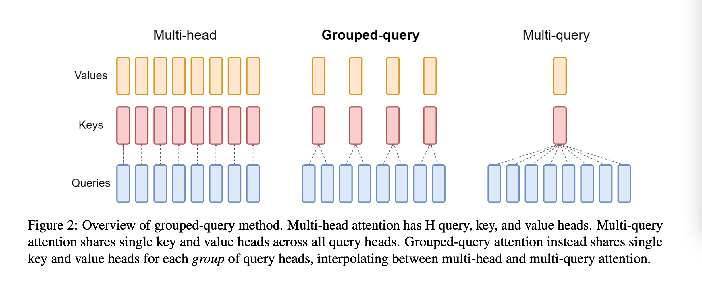
2023年，论文《GQA: Training Generalized Multi-Query Transformer Models from Multi-Head Checkpoints》 提出Grouped-Query Attention（分组注意力），来平衡效率和性能。通过将查询头分组，组内共享键和值矩阵，从而减少计算量。具体步骤如下：

1. 头分组：将 $h$ 个查询头分为 $g$ 组，每组 $h/g$ 个头。
2. 共享参数：每组共享键和值矩阵 $K_g,V_g$。
3. 注意力计算：
   GroupedAttention ( Q , { K g , V g } ) = Concat ( head 1 , … , head g ) \text{GroupedAttention}(Q, \{K_g, V_g\}) = \text{Concat}(\text{head}_1, \dots, \text{head}_g) GroupedAttention(Q,{Kg​,Vg​})=Concat(head1​,…,headg​)
   其中 ${\text{head}}_g=\text{Attention}(Q_g,K_g,V_g)$。

Meta 的 LLaMA 2 采用此机制GQA，在保持性能的同时减少内存占用。你可能会想，既然可以分成多组，可不只分成一组（所有头共享同一组键和值），那样计算效率应该跟高。其实论文也实验了这种方法Multi-Query Attention (MQA)，但表达能力较弱。下图展示了 MHA、GQA、MQA的网络结构：

Grouped-Query Attention在性能优化方面的表示也十分出色。首先，内存节省：键值矩阵的存储量从 $O(h\cdot n\cdot d)$ 降至 $O(g\cdot n\cdot d)$。 其次，计算加速：矩阵乘法次数减少 $h/g$ 倍。

5.2 代码

class GroupedAttention(nn.Module):
    def __init__(self, input_dim, d_k, num_heads, num_groups):
        super(GroupedAttention, self).__init__()
        assert num_heads % num_groups == 0
        self.num_heads = num_heads
        self.num_groups = num_groups
        self.head_dim = d_k // num_heads
        self.W_q = nn.Linear(input_dim, d_k)
        self.W_k = nn.Linear(input_dim, d_k // num_groups)
        self.W_v = nn.Linear(input_dim, d_k // num_groups)
        self.W_o = nn.Linear(d_k, input_dim)

    def forward(self, x):
        batch_size, seq_len, _ = x.size()
        Q = self.W_q(x).view(batch_size, seq_len, self.num_heads, self.head_dim).transpose(1, 2)
        K = self.W_k(x).view(batch_size, seq_len, self.num_heads // self.num_groups, self.head_dim).transpose(1, 2)
        V = self.W_v(x).view(batch_size, seq_len, self.num_heads // self.num_groups, self.head_dim).transpose(1, 2)
        # 调整 Q 的形状以匹配 K 的分组
        Q = Q.view(batch_size, self.num_groups, self.num_heads // self.num_groups, seq_len, self.head_dim)
        scores = torch.matmul(Q, K.transpose(-2, -1)) / torch.sqrt(torch.tensor(self.head_dim).float())
        attn_weights = F.softmax(scores, dim=-1)
        output = torch.matmul(attn_weights, V)
        output = output.view(batch_size, self.num_heads, seq_len, self.head_dim).transpose(1, 2).contiguous().view(batch_size, seq_len, -1)
        output = self.W_o(output)
        return output

---

6. Tensor Product Attention

6.1 原理

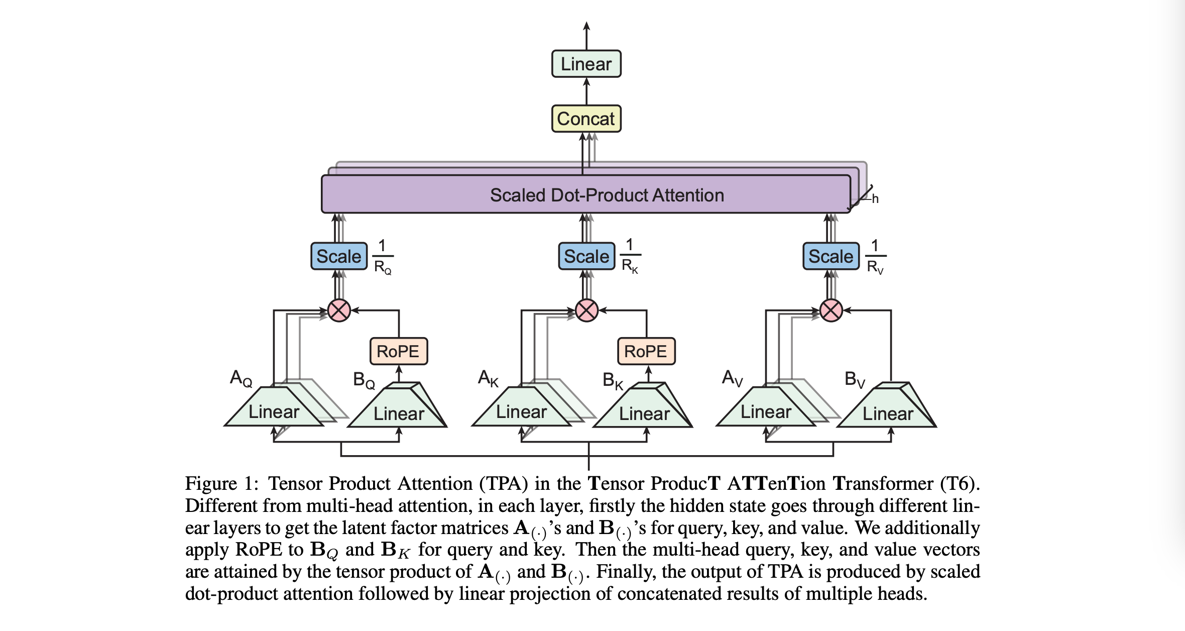
2025年，论文《TPA：Tensor Product Attention Is All You Need》提出 Tensor Product Attention（张量积注意力），通过动态分解查询、键、值矩阵，显著减少内存占用。

TPA 是一种通过张量分解实现高效注意力计算的机制，核心思想是将查询（Q）、键（K）、值（V）动态分解为低秩张量的外积之和，从而压缩内存占用并提升长序列处理效率。具体原理如下：

1. 张量分解机制

对于查询（Q）、键（K）、值（V）矩阵，TPA 将每个令牌的表示动态分解为低秩张量外积的加权和。以查询矩阵 $Q$ 为例，其分解公式为：
$$Q_t=\frac{1}{R_Q}\sum _{r=1}^{R_Q}{a}_r^Q(x_t)\otimes b_r^Q(x_t)$$
其中：

• $Q_t$ 是第 $t$ 个令牌的查询矩阵表示。
• $R_Q$ 是查询矩阵的分解秩，代表分解中所使用的低秩分量的数量。
• $\otimes$ 表示外积运算。
• $a_r^Q(x_t)\in {\mathbb{R}}^h$ 是头维度向量，$h$ 是头的维度，它是输入 $x_t$ 的线性变换结果。
• $b_r^Q(x_t)\in {\mathbb{R}}^{d_h}$ 是令牌维度向量，$d_h$ 是每个头的维度，同样是输入 $x_t$ 的线性变换结果。
• 上下文依赖：$a_r^Q,b_r^Q$ 是输入 $x_t$ 的线性变换结果，实现动态上下文感知的低秩表示。

键矩阵 $K$ 和值矩阵 $V$ 也采用类似的分解方式：
$$K_t=\frac{1}{R_K}\sum _{r=1}^{R_K}{a}_r^K(x_t)\otimes b_r^K(x_t)$$
$$V_t=\frac{1}{R_V}\sum _{r=1}^{R_V}{a}_r^V(x_t)\otimes b_r^V(x_t)$$
这里 $R_K$ 和 $R_V$ 分别是键矩阵和值矩阵的分解秩。

特点:

• 1. 动态上下文感知：分解中的 $a_r^Q$、$b_r^Q$、$a_r^K$、$b_r^K$、$a_r^V$ 和 $b_r^V$ 都是输入 $x_t$ 的线性变换结果，这意味着分解是动态的，能够根据输入的不同上下文进行调整，从而实现上下文感知的低秩表示。
• 2. 低秩表示：通过将矩阵分解为低秩张量的外积之和，减少了存储和计算所需的参数数量，从而降低了内存占用和计算复杂度。在实际应用中，当 $R_Q$、$R_K$ 和 $R_V$ 远小于头维度 $h$ 时，能够显著节省内存。
• 3. 与位置编码兼容性：TPA 能够与旋转位置编码（RoPE）兼容，通过对令牌维度向量 $b_r^Q$ 和 $b_r^K$ 应用 RoPE 旋转操作，保持了相对位置信息，使得模型在处理序列时能够考虑到元素之间的相对位置关系。

与传统矩阵分解的区别:
传统的矩阵分解方法，如奇异值分解（SVD）、特征分解等，通常是静态的，分解结果不依赖于输入数据的上下文。而 TPA 中的矩阵分解是动态的，其分解结果会根据输入的不同而变化，更适合处理具有上下文信息的序列数据。这种动态分解方式使得 TPA 在处理长序列数据时具有更好的性能和效率。

2. RoPE 兼容性

• 位置编码整合：通过对令牌维度向量 $b_r^Q,b_r^K$ 应用 RoPE 旋转操作，保持相对位置信息：
  $$\text{RoPE}(Q_t)=\frac{1}{R_Q}{A}_Q(x_t{)}^{\top }\cdot \text{RoPE}(B_Q(x_t))$$
  其中 $A_Q,B_Q$ 分别为头维度和令牌维度的分解矩阵，确保位置编码与张量分解无缝结合。

3. 内存优化

• KV 缓存压缩：仅存储分解后的低秩因子 $A_K,B_K,A_V,B_V$，而非完整的 K、V 矩阵。内存占用从标准注意力的 $O(Th{d}_h)$ 降至 $O(T(R_K+R_V)(h+d_h))$，当 $R_K,R_V\ll h$ 时，内存节省可达 10 倍以上。

其网络结构如下图：

6.2 代码

class TensorProductAttention(nn.Module):
    def __init__(
        self,
        d_model: int,        # 输入维度
        num_heads: int,      # 注意力头数
        d_k: int,            # 每个头的维度
        r_q: int = 6,        # 查询分解秩
        r_k: int = 2,        # 键分解秩
        r_v: int = 2         # 值分解秩
    ):
        super(TensorProductAttention, self).__init__()
        self.num_heads = num_heads
        self.d_k = d_k
        self.r_q, self.r_k, self.r_v = r_q, r_k, r_v

        # 分解矩阵：头维度 (h) 和 令牌维度 (d_k) 的线性层
        self.W_a_q = nn.Linear(d_model, num_heads * r_q)     # 头维度因子 (A_Q)
        self.W_b_q = nn.Linear(d_model, d_k * r_q)          # 令牌维度因子 (B_Q)
        self.W_a_k = nn.Linear(d_model, num_heads * r_k)     # A_K
        self.W_b_k = nn.Linear(d_model, d_k * r_k)          # B_K
        self.W_a_v = nn.Linear(d_model, num_heads * r_v)     # A_V
        self.W_b_v = nn.Linear(d_model, d_k * r_v)          # B_V

        self.out_proj = nn.Linear(num_heads * d_k, d_model)  # 输出投影层

    def forward(self, x: torch.Tensor, rope_pos: torch.Tensor = None):
        batch_size, seq_len, _ = x.shape

        # 生成分解因子 (A, B)
        # Q: (batch, seq, r_q*h) -> (batch, seq, r_q, h)
        A_Q = self.W_a_q(x).view(batch_size, seq_len, self.r_q, self.num_heads).transpose(1, 2)
        B_Q = self.W_b_q(x).view(batch_size, seq_len, self.r_q, self.d_k).transpose(1, 2)
        # K: (batch, seq, r_k*h) -> (batch, seq, r_k, h)
        A_K = self.W_a_k(x).view(batch_size, seq_len, self.r_k, self.num_heads).transpose(1, 2)
        B_K = self.W_b_k(x).view(batch_size, seq_len, self.r_k, self.d_k).transpose(1, 2)
        # V: (batch, seq, r_v*h) -> (batch, seq, r_v, h)
        A_V = self.W_a_v(x).view(batch_size, seq_len, self.r_v, self.num_heads).transpose(1, 2)
        B_V = self.W_b_v(x).view(batch_size, seq_len, self.r_v, self.d_k).transpose(1, 2)

        # 应用 RoPE（假设 rope_pos 为位置相关的旋转矩阵）
        if rope_pos is not None:
            # 调整 rope_pos 的形状以匹配 B_Q 和 B_K
            rope_pos = rope_pos.unsqueeze(0).unsqueeze(1)  # 形状变为 (1, 1, seq_len, d_k)
            B_Q = B_Q * rope_pos
            B_K = B_K * rope_pos

        # 重构 Q, K, V
        Q = (A_Q.unsqueeze(-1) * B_Q.unsqueeze(-2)).sum(dim=1)  # (batch, seq, h, d_k)
        K = (A_K.unsqueeze(-1) * B_K.unsqueeze(-2)).sum(dim=1)  # (batch, seq, h, d_k)
        V = (A_V.unsqueeze(-1) * B_V.unsqueeze(-2)).sum(dim=1)  # (batch, seq, h, d_k)

        # 注意力计算：(batch, seq, h, d_k) @ (batch, seq, d_k, h) -> (batch, h, seq, seq)  。后面的结构与self-attention还是一致
        scores = (Q @ K.transpose(2, 3)) / torch.sqrt(torch.tensor(self.d_k, dtype=torch.float32))
        attn_weights = F.softmax(scores, dim=-1)
        output = (attn_weights @ V).transpose(1, 2).contiguous()  # (batch, seq, h, d_k)

        # 拼接头并投影
        output = output.view(batch_size, seq_len, -1)
        return self.out_proj(output)

1. 代码说明

• 张量分解：通过线性层将输入映射为低秩因子 $A,B$，分别对应头维度和令牌维度的表示。
• RoPE 集成：在令牌维度向量 $B_Q,B_K$ 上应用位置编码，保持相对位置信息（具体旋转矩阵需根据 RoPE 公式实现）。
• 注意力计算：利用分解后的 Q、K 计算分数，通过 Softmax 生成权重，再与 V 加权求和。

2. 输出说明

• 输出维度：与输入维度一致，保持模型结构兼容性。
• 内存占用：相比标准注意力，KV 缓存大小从 $2\times 1024\times 12\times 64=1572864$ 降至 $2\times 1024\times (2+2)\times (12+64)=589824$，节省约 63% 内存。

3. 核心优势

1. 内存效率：通过低秩分解大幅减少 KV 缓存，支持更长序列处理（论文表 1 显示 KV 缓存减少 10×以上）。
2. 性能提升：在语言建模任务中，TPA 比 MHA、GQA 等基线模型实现更低困惑度（Perplexity）和更高下游任务准确率（论文图 2-4、表 2-3）。
3. RoPE 兼容性：通过令牌维度向量旋转，无缝集成位置编码，保持相对位置信息（论文定理 1、3.2 节）。

TPA通过参数配置支持不同分解秩和头数，适用于长上下文场景如文档分析、代码生成等。实际部署时可结合硬件优化（如 CUDA 核融合）进一步提升效率。具体代码实现，还可以参考官方代码（https://github.com/tensorgi/T6）

---

7. FlashAttention

7.1 原理

FlashAttention 是一种通用的加速方法，所以他是一种硬件优化技术，并非前面提到的网络结构算法。理论上可以应用于大模型（如 GPT、BERT）以及 Stable Diffusion（SD）等需要使用 Attention 计算的模型。但它的适用性和效果取决于模型的具体实现以及 FlashAttention 的特性。FlashAttention 通过以下策略实现高效计算：

1. 分块计算（Tiling）：

   • 将输入矩阵划分为小块，逐块加载到 SRAM 中计算。
   • 减少 HBM 与 SRAM 之间的读写次数。

2. 重计算（Recomputation）：

   • 前向计算时不存储中间矩阵，后向传播时重新计算。
   • 内存占用从 $O(n^2)$ 降至 $O(n)$。

3. 块稀疏注意力：

   • 仅计算非零块的注意力，进一步减少计算量。

---

8 对比

机制	核心优势	典型应用场景	局限性
Self-Attention	全局依赖建模	NLP 序列处理	时间复杂度高
Spatial Attention	空间聚焦	计算机视觉	忽略通道间关系
Temporal Attention	时序动态建模	视频、语音	依赖位置编码
Cross-Attention	跨模态交互	多模态任务	需成对输入
Grouped Attention	计算效率高	大模型推理	可能损失表达能力
Tensor Product Attention	内存高效	超长序列处理	实现复杂度高
FlashAttention	长序列加速	大模型训练	硬件依赖（如 GPU）

---

9 测试代码

代码：

import torch
import torch.nn as nn
import torch.nn.functional as F


# 1. Self-Attention
class SelfAttention(nn.Module):
    def __init__(self, input_dim, d_k):
        super(SelfAttention, self).__init__()
        self.W_q = nn.Linear(input_dim, d_k)
        self.W_k = nn.Linear(input_dim, d_k)
        self.W_v = nn.Linear(input_dim, d_k)

    def forward(self, x):
        Q = self.W_q(x)
        K = self.W_k(x)
        V = self.W_v(x)
        scores = torch.matmul(Q, K.transpose(-2, -1)) / torch.sqrt(torch.tensor(Q.size(-1)).float())
        attn_weights = F.softmax(scores, dim=-1)
        output = torch.matmul(attn_weights, V)
        return output



# 1.2 MHA
class MultiHeadAttention(nn.Module):
    def __init__(self, input_dim, num_heads, d_k):
        super(MultiHeadAttention, self).__init__()
        self.input_dim = input_dim
        self.num_heads = num_heads
        self.d_k = d_k
        self.head_dim = d_k // num_heads

        # 线性层用于生成 Q, K, V
        self.W_q = nn.Linear(input_dim, d_k)
        self.W_k = nn.Linear(input_dim, d_k)
        self.W_v = nn.Linear(input_dim, d_k)
        self.W_o = nn.Linear(d_k, input_dim)

    def forward(self, x):
        batch_size, seq_len, _ = x.size()

        # 生成 Q, K, V
        Q = self.W_q(x).view(batch_size, seq_len, self.num_heads, self.head_dim).transpose(1, 2)
        K = self.W_k(x).view(batch_size, seq_len, self.num_heads, self.head_dim).transpose(1, 2)
        V = self.W_v(x).view(batch_size, seq_len, self.num_heads, self.head_dim).transpose(1, 2)

        # 计算注意力分数
        scores = torch.matmul(Q, K.transpose(-2, -1)) / torch.sqrt(torch.tensor(self.head_dim).float())
        attn_weights = F.softmax(scores, dim=-1)

        # 计算加权和
        output = torch.matmul(attn_weights, V)
        output = output.transpose(1, 2).contiguous().view(batch_size, seq_len, -1)

        # 输出投影
        output = self.W_o(output)
        return output




# 2. Spatial Attention
class SpatialAttention(nn.Module):
    def __init__(self, kernel_size=7):
        super(SpatialAttention, self).__init__()
        assert kernel_size in (3, 7), 'kernel size must be 3 or 7'
        padding = 3 if kernel_size == 7 else 1
        self.conv1 = nn.Conv2d(2, 1, kernel_size, padding=padding, bias=False)
        self.sigmoid = nn.Sigmoid()

    def forward(self, x):
        avg_out = torch.mean(x, dim=1, keepdim=True)
        max_out, _ = torch.max(x, dim=1, keepdim=True)
        x = torch.cat([avg_out, max_out], dim=1)
        x = self.conv1(x)
        return self.sigmoid(x)


# 3. Temporal Attention
class TemporalAttention(nn.Module):
    def __init__(self, input_dim, d_k, time_emb_dim):
        super(TemporalAttention, self).__init__()
        self.input_dim = input_dim  # 输入文本嵌入维度
        self.d_k = d_k  # Q/K/V维度
        self.time_emb_dim = time_emb_dim  # 时间嵌入维度
        
        # 文本的Q/K/V线性层
        self.W_q = nn.Linear(input_dim, d_k)
        self.W_k = nn.Linear(input_dim, d_k)
        self.W_v = nn.Linear(input_dim, d_k)
        
        # 时间嵌入的线性层（将时间点映射到d_k维度）
        self.W_t = nn.Linear(time_emb_dim, d_k)
    
    def forward(self, x, time_points):
        batch_size, seq_len, _ = x.size()
        num_time_points = time_points.size(1)  # 假设每个序列对应一个时间点
        
        # 生成文本的Q/K/V
        Q = self.W_q(x)  # (batch_size, seq_len, d_k)
        K = self.W_k(x)  # (batch_size, seq_len, d_k)
        V = self.W_v(x)  # (batch_size, seq_len, d_k)
        
        # 生成时间矩阵T：将时间点嵌入扩展为序列长度一致的矩阵
        time_emb = self.W_t(time_points)  # (batch_size, 1, d_k)
        T = time_emb.repeat(1, seq_len, 1)  # (batch_size, seq_len, d_k)
        
        # 计算时间矩阵的全局范数（Frobenius范数）
        T_norm = torch.norm(T, p='fro', dim=(1, 2), keepdim=True)  # (batch_size, 1, 1)
        T_scaled = (T.transpose(1, 2) @ T) / (T_norm + 1e-8)  # (batch_size, d_k, d_k)
                                                             # a @ b 就相当于 torch.matmul(a, b)
        
        # 计算注意力分数：Q * T_scaled * K^T
        scores = torch.matmul(Q, T_scaled)  # (batch_size, seq_len, d_k)
        scores = torch.matmul(scores, K.transpose(1, 2))  # (batch_size, seq_len, seq_len)
        scores = scores / torch.sqrt(torch.tensor(self.d_k, dtype=torch.float32))
        
        # 归一化和加权求和
        attn_weights = F.softmax(scores, dim=-1)
        output = torch.matmul(attn_weights, V)
        return output, attn_weights



# 4. Cross-Attention
class CrossAttention(nn.Module):
    def __init__(self, input_dim, d_k):
        super(CrossAttention, self).__init__()
        self.W_q = nn.Linear(input_dim, d_k)
        self.W_k = nn.Linear(input_dim, d_k)
        self.W_v = nn.Linear(input_dim, d_k)

    def forward(self, x1, x2):
        Q = self.W_q(x1)
        K = self.W_k(x2)
        V = self.W_v(x2)
        scores = torch.matmul(Q, K.transpose(-2, -1)) / torch.sqrt(torch.tensor(Q.size(-1)).float())
        attn_weights = F.softmax(scores, dim=-1)
        output = torch.matmul(attn_weights, V)
        return output


# 5. Grouped Attention
class GroupedAttention(nn.Module):
    def __init__(self, input_dim, d_k, num_heads, num_groups):
        super(GroupedAttention, self).__init__()
        assert num_heads % num_groups == 0
        self.num_heads = num_heads
        self.num_groups = num_groups
        self.head_dim = d_k // num_heads
        self.W_q = nn.Linear(input_dim, d_k)
        self.W_k = nn.Linear(input_dim, d_k // num_groups)
        self.W_v = nn.Linear(input_dim, d_k // num_groups)
        self.W_o = nn.Linear(d_k, input_dim)

    def forward(self, x):
        batch_size, seq_len, _ = x.size()
        Q = self.W_q(x).view(batch_size, seq_len, self.num_heads, self.head_dim).transpose(1, 2)
        K = self.W_k(x).view(batch_size, seq_len, self.num_heads // self.num_groups, self.head_dim).transpose(1, 2)
        V = self.W_v(x).view(batch_size, seq_len, self.num_heads // self.num_groups, self.head_dim).transpose(1, 2)
        # 调整 Q 的形状以匹配 K 的分组
        Q = Q.view(batch_size, self.num_groups, self.num_heads // self.num_groups, seq_len, self.head_dim)
        scores = torch.matmul(Q, K.transpose(-2, -1)) / torch.sqrt(torch.tensor(self.head_dim).float())
        attn_weights = F.softmax(scores, dim=-1)
        output = torch.matmul(attn_weights, V)
        output = output.view(batch_size, self.num_heads, seq_len, self.head_dim).transpose(1, 2).contiguous().view(batch_size, seq_len, -1)
        output = self.W_o(output)
        return output


# 6. Tensor Product Attention
class TensorProductAttention(nn.Module):
    def __init__(
        self,
        d_model: int,        # 输入维度
        num_heads: int,      # 注意力头数
        d_k: int,            # 每个头的维度
        r_q: int = 6,        # 查询分解秩
        r_k: int = 2,        # 键分解秩
        r_v: int = 2         # 值分解秩
    ):
        super(TensorProductAttention, self).__init__()
        self.num_heads = num_heads
        self.d_k = d_k
        self.r_q, self.r_k, self.r_v = r_q, r_k, r_v

        # 分解矩阵：头维度 (h) 和 令牌维度 (d_k) 的线性层
        self.W_a_q = nn.Linear(d_model, num_heads * r_q)     # 头维度因子 (A_Q)
        self.W_b_q = nn.Linear(d_model, d_k * r_q)          # 令牌维度因子 (B_Q)
        self.W_a_k = nn.Linear(d_model, num_heads * r_k)     # A_K
        self.W_b_k = nn.Linear(d_model, d_k * r_k)          # B_K
        self.W_a_v = nn.Linear(d_model, num_heads * r_v)     # A_V
        self.W_b_v = nn.Linear(d_model, d_k * r_v)          # B_V

        self.out_proj = nn.Linear(num_heads * d_k, d_model)  # 输出投影层

    def forward(self, x: torch.Tensor, rope_pos: torch.Tensor = None):
        batch_size, seq_len, _ = x.shape

        # 生成分解因子 (A, B)
        # Q: (batch, seq, r_q*h) -> (batch, seq, r_q, h)
        A_Q = self.W_a_q(x).view(batch_size, seq_len, self.r_q, self.num_heads).transpose(1, 2)
        B_Q = self.W_b_q(x).view(batch_size, seq_len, self.r_q, self.d_k).transpose(1, 2)
        # K: (batch, seq, r_k*h) -> (batch, seq, r_k, h)
        A_K = self.W_a_k(x).view(batch_size, seq_len, self.r_k, self.num_heads).transpose(1, 2)
        B_K = self.W_b_k(x).view(batch_size, seq_len, self.r_k, self.d_k).transpose(1, 2)
        # V: (batch, seq, r_v*h) -> (batch, seq, r_v, h)
        A_V = self.W_a_v(x).view(batch_size, seq_len, self.r_v, self.num_heads).transpose(1, 2)
        B_V = self.W_b_v(x).view(batch_size, seq_len, self.r_v, self.d_k).transpose(1, 2)

        # 应用 RoPE（假设 rope_pos 为位置相关的旋转矩阵）
        if rope_pos is not None:
            # 调整 rope_pos 的形状以匹配 B_Q 和 B_K
            rope_pos = rope_pos.unsqueeze(0).unsqueeze(1)  # 形状变为 (1, 1, seq_len, d_k)
            B_Q = B_Q * rope_pos
            B_K = B_K * rope_pos

        # 重构 Q, K, V
        Q = (A_Q.unsqueeze(-1) * B_Q.unsqueeze(-2)).sum(dim=1)  # (batch, seq, h, d_k)
        K = (A_K.unsqueeze(-1) * B_K.unsqueeze(-2)).sum(dim=1)  # (batch, seq, h, d_k)
        V = (A_V.unsqueeze(-1) * B_V.unsqueeze(-2)).sum(dim=1)  # (batch, seq, h, d_k)

        # 注意力计算：(batch, seq, h, d_k) @ (batch, seq, d_k, h) -> (batch, h, seq, seq)
        scores = (Q @ K.transpose(2, 3)) / torch.sqrt(torch.tensor(self.d_k, dtype=torch.float32))
        attn_weights = F.softmax(scores, dim=-1)
        output = (attn_weights @ V).transpose(1, 2).contiguous()  # (batch, seq, h, d_k)

        # 拼接头并投影
        output = output.view(batch_size, seq_len, -1)
        return self.out_proj(output)



# 测试代码
if __name__ == "__main__":
    # ======== 测试 Self-Attention
    input_dim = 64
    d_k = 32
    seq_len = 10
    batch_size = 2

    x = torch.randn(batch_size, seq_len, input_dim)
    self_attn = SelfAttention(input_dim, d_k)
    output_self = self_attn(x)
    print("Self-Attention output shape:", output_self.shape)


    # ======== 测试 MHA
    num_heads = 4
    input_dim = 64
    d_k = 32
    seq_len = 10
    batch_size = 2

    x = torch.randn(batch_size, seq_len, input_dim)
    mha = MultiHeadAttention(input_dim, num_heads, d_k)
    output = mha(x)
    print("Multi-Head Attention output shape:", output.shape)
    

    # ======== 测试 Spatial Attention
    channels = 3
    height = 16
    width = 16

    x_spatial = torch.randn(batch_size, channels, height, width)

    spatial_attn = SpatialAttention()
    attn_map = spatial_attn(x_spatial)
    output_spatial = x_spatial * attn_map
    print("Spatial-Attention output shape:", output_spatial.shape)

    # ======== 测试 Temporal Attention
    # 超参数
    input_dim = 768  # BERT词嵌入维度
    d_k = 64  # Q/K/V维度
    time_emb_dim = 32  # 时间嵌入维度
    batch_size = 2
    seq_len = 10
    
    # 输入：文本嵌入和时间点（每个序列对应一个时间点，维度为(batch_size, 1, time_emb_dim)）
    x = torch.randn(batch_size, seq_len, input_dim)
    time_points = torch.randn(batch_size, 1, time_emb_dim)  # 例如时间戳的嵌入

    temporal_attn = TemporalAttention(input_dim, d_k, time_emb_dim)
    output_temporal, attn_weights = temporal_attn(x, time_points)
    print("Temporal-Attention output shape:", output_temporal.shape) # 应输出(batch_size, seq_len, d_k)

    # ======== 测试 Cross-Attention
    x1 = torch.randn(batch_size, seq_len, input_dim)
    x2 = torch.randn(batch_size, seq_len, input_dim)
    cross_attn = CrossAttention(input_dim, d_k)
    output_cross = cross_attn(x1, x2)
    print("Cross-Attention output shape:", output_cross.shape)

    # ======== 测试 Grouped Attention
    num_heads = 4
    num_groups = 2
    grouped_attn = GroupedAttention(input_dim, d_k, num_heads, num_groups)
    output_grouped = grouped_attn(x)
    print("Grouped-Attention output shape:", output_grouped.shape)


    # ======== 测试 Tensor Product Attention
    # 超参数
    d_model = 768       # 输入维度（如 BERT-base）
    num_heads = 12      # 注意力头数
    d_k = 64            # 每个头的维度
    r_q, r_k, r_v = 6, 2, 2  # 分解秩（论文默认配置）
    batch_size, seq_len = 2, 1024  # 批次大小和序列长度

    # 输入数据：(batch_size, seq_len, d_model)
    x = torch.randn(batch_size, seq_len, d_model)
    # RoPE 位置编码（示例：简化的正弦编码，实际需匹配模型）
    rope_pos = torch.randn(seq_len, d_k)

    tpa = TensorProductAttention(d_model, num_heads, d_k, r_q, r_k, r_v)
    output_tpa = tpa(x, rope_pos)

    # 验证输出形状：(batch_size, seq_len, d_model)
    print("Tensor Product Attention output shape:", output_tpa.shape)  # 应输出 (2, 1024, 768)

执行结果：

Self-Attention output shape: torch.Size([2, 10, 32])
Multi-Head Attention output shape: torch.Size([2, 10, 64])
Spatial-Attention output shape: torch.Size([2, 3, 16, 16])
Temporal-Attention output shape: torch.Size([2, 10, 64])
Cross-Attention output shape: torch.Size([2, 10, 64])
Grouped-Attention output shape: torch.Size([2, 10, 768])
Tensor Product Attention output shape: torch.Size([2, 1024, 768])

引用

[1]. Attention Is All You Need

[2]. Swin Transformer: Hierarchical Vision Transformer using Shifted Windows

[3]. CBAM: Convolutional Block Attention Module

[4]. Temporal Attention for Language Models

[5]. Tensor Product Attention Is All You Need

[6]. Introduction to Attention Mechanism