Dive into Deep Learning - 2.4. Calculus {微积分}
- 1. Derivatives and Differentiation (导数和微分)
- 1.1. Visualization Utilities
- 2. Chain Rule (链式法则)
- 3. Discussion
- References
2.4. Calculus
https://d2l.ai/chapter_preliminaries/calculus.html
For a long time, how to calculate the area of a circle remained a mystery. Then, in Ancient Greece, the mathematician Archimedes came up with the clever idea to inscribe a series of polygons with increasing numbers of vertices on the inside of a circle.
inscribe /ɪnˈskraɪb/ vt. 题写;题献;铭记;雕
For a polygon with n n n vertices, we obtain n n n triangles. The height of each triangle approaches the radius r r r as we partition the circle more finely. At the same time, its base approaches 2 π r / n 2 \pi r/n 2πr/n, since the ratio between arc and secant approaches 1 for a large number of vertices. Thus, the area of the polygon approaches 1 2 ⋅ ( 2 π r / n ) ⋅ r ⋅ n = π r 2 \frac{1}{2} \cdot (2 \pi r/n) \cdot r \cdot n = \pi r^2 21⋅(2πr/n)⋅r⋅n=πr2.
arc /ɑːk/ n. 弧度;弧形物;天穹;弧光 (electric arc) adj. 圆弧的;反三角函数的 vt. 走弧线;形成电弧
secant /'siːk(ə)nt/ adj. 割的;切的;交叉的 n. 割线;正割
古希腊人把一个多边形分成三角形,并把它们的面积相加,计算多边形的面积。为了求出圆的面积,古希腊人在圆内接多边形。内接多边形的等长边越多,就越接近圆。 这个过程也被称为逼近法 (method of exhaustion)。

Fig. 1 Finding the area of a circle as a limit procedure.
This limiting procedure is at the root of both differential calculus and integral calculus.
微分和积分是微积分的两个分支,微分可以应用于深度学习中的优化问题。
calculus /'kælkjʊləs/ n. 微积分 (学),结石,积石
integral calculus 积分学
differential calculus 微分学
在深度学习中,我们训练模型,并不断更新它们,使它们在看到越来越多的数据时变得越来越好。通常情况下,变得更好意味着最小化一个损失函数 (loss function),即一个衡量“模型有多糟糕”这个问题的分数。我们真正关心的是生成一个模型,它能够在从未见过的数据上表现良好。但训练模型只能将模型与我们实际能看到的数据相拟合。因此,我们可以将拟合模型的任务分解为两个关键问题:
- 优化 (optimization):用模型拟合观测数据的过程。
- 泛化 (generalization):生成出有效性超出用于训练的数据集本身的模型。
1. Derivatives and Differentiation (导数和微分)
Put simply, a derivative is the rate of change in a function with respect to changes in its arguments. Derivatives can tell us how rapidly a loss function would increase or decrease were we to increase or decrease each parameter by an infinitesimally small amount.
在深度学习中,我们通常选择对于模型参数可微的损失函数。对于每个参数,如果我们把这个参数增加或减少一个无穷小的量,可以知道损失会以多快的速度增加或减少。
Formally, for functions
f
:
R
→
R
f: \mathbb{R} \rightarrow \mathbb{R}
f:R→R, that map from scalars to scalars (其输入和输出都是标量), the derivative of
f
f
f at a point
x
x
x is defined as
f
′
(
x
)
=
lim
h
→
0
f
(
x
+
h
)
−
f
(
x
)
h
.
f'(x) = \lim_{h \rightarrow 0} \frac{f(x+h) - f(x)}{h}.
f′(x)=h→0limhf(x+h)−f(x).
This term on the right hand side is called a limit and it tells us what happens to the value of an expression as a specified variable approaches a particular value. This limit tells us what the ratio between a perturbation h h h and the change in the function value f ( x + h ) − f ( x ) f(x + h) - f(x) f(x+h)−f(x) converges to as we shrink its size to zero.
perturbation /ˌpɜːtə'beɪʃ(ə)n/ n. 忧虑;不安;烦恼;摄动;微扰;小变异
When
f
′
(
x
)
f'(x)
f′(x) exists,
f
f
f is said to be differentiable at
x
x
x; and when
f
′
(
x
)
f'(x)
f′(x) exists for all
x
x
x on a set, e.g., the interval
[
a
,
b
]
[a,b]
[a,b], we say that
f
f
f is differentiable on this set.
如果
f
′
(
a
)
f'(a)
f′(a) 存在,则称
f
f
f 在
a
a
a 处是可微 (differentiable) 的。如果
f
f
f 在一个区间内的每个数上都是可微的,则此函数在此区间中是可微的。
Not all functions are differentiable, including many that we wish to optimize, such as accuracy and the area under the receiving operating characteristic (AUC). However, because computing the derivative of the loss is a crucial step in nearly all algorithms for training deep neural networks, we often optimize a differentiable surrogate instead.
由于计算损失的导数是几乎所有训练深度神经网络算法的关键步骤,因此我们通常会优化可微分的替代函数。
surrogate /ˈsʌrəɡət/ adj. 替代的,代理的 n. 代理人;主教代理人;遗嘱检验法官 v. 取代,替代;指定 (某人) 为自己的代理人
We can interpret the derivative
f
′
(
x
)
f'(x)
f′(x) as the instantaneous rate of change of
f
(
x
)
f(x)
f(x) with respect to
x
x
x.
导数
f
′
(
x
)
f'(x)
f′(x) 解释为
f
(
x
)
f(x)
f(x) 相对于
x
x
x 的瞬时 (instantaneous) 变化率。所谓的瞬时变化率是基于
x
x
x 中的变化
h
h
h,且
h
h
h 接近
0
0
0。
Let’s develop some intuition with an example. Define u = f ( x ) = 3 x 2 − 4 x u = f(x) = 3x^2-4x u=f(x)=3x2−4x.
Setting
x
=
1
x=1
x=1, we see that
f
(
x
+
h
)
−
f
(
x
)
h
\frac{f(x+h) - f(x)}{h}
hf(x+h)−f(x) approaches
2
2
2 as
h
h
h approaches
0
0
0. While this experiment lacks the rigor of a mathematical proof, we can quickly see that indeed
f
′
(
1
)
=
2
f'(1) = 2
f′(1)=2.
通过令
x
=
1
x=1
x=1 并让
h
h
h 接近
0
0
0,
f
(
x
+
h
)
−
f
(
x
)
h
\frac{f(x+h)-f(x)}{h}
hf(x+h)−f(x) 的数值结果接近
2
2
2。虽然这个实验不是一个数学证明,但稍后会看到,当
x
=
1
x=1
x=1 时,导数
u
′
u'
u′ 是
2
2
2。
rigor /ˈrɪɡə/ n. 严格,严厉;严谨,严密;严酷;艰苦;(发热前的) 寒战;(由惊吓或中毒等导致的身体) 僵直,强直
#!/usr/bin/env python
# coding=utf-8

def f(x):
    return 3 * (x ** 2) - 4 * x


def numerical_lim(f, x, h):
    return (f(x + h) - f(x)) / h


h = 0.1
for i in range(5):
    print(f'h={h:.5f}, numerical limit={numerical_lim(f, 1, h):.5f}')
    h *= 0.1
/home/yongqiang/miniconda3/bin/python /home/yongqiang/stable_diffusion_work/stable_diffusion_diffusers/yongqiang.py
h=0.10000, numerical limit=2.30000
h=0.01000, numerical limit=2.03000
h=0.00100, numerical limit=2.00300
h=0.00010, numerical limit=2.00030
h=0.00001, numerical limit=2.00003

Process finished with exit code 0
There are several equivalent notational conventions for derivatives. Given y = f ( x ) y = f(x) y=f(x), the following expressions are equivalent:
f ′ ( x ) = y ′ = d y d x = d f d x = d d x f ( x ) = D f ( x ) = D x f ( x ) , f'(x) = y' = \frac{dy}{dx} = \frac{df}{dx} = \frac{d}{dx} f(x) = Df(x) = D_x f(x), f′(x)=y′=dxdy=dxdf=dxdf(x)=Df(x)=Dxf(x),
where the symbols
d
d
x
\frac{d}{dx}
dxd and
D
D
D are differentiation operators.
其中符号
d
d
x
\frac{d}{dx}
dxd 和
D
D
D是 微分运算符,表示微分操作。
Below, we present the derivatives of some common functions:
d d x C = 0 for any constant C d d x x n = n x n − 1 for n ≠ 0 d d x e x = e x d d x ln x = x − 1 . \begin{aligned} \frac{d}{dx} C & = 0 && \textrm{for any constant $C$} \\ \frac{d}{dx} x^n & = n x^{n-1} && \textrm{for } n \neq 0 \\ \frac{d}{dx} e^x & = e^x \\ \frac{d}{dx} \ln x & = x^{-1}. \end{aligned} dxdCdxdxndxdexdxdlnx=0=nxn−1=ex=x−1.for any constant Cfor n=0
- D C = 0 DC = 0 DC=0( C C C是一个常数)
- D x n = n x n − 1 Dx^n = nx^{n-1} Dxn=nxn−1( n n n 是任意实数)
- D e x = e x De^x = e^x Dex=ex
- D ln ( x ) = 1 / x D\ln(x) = 1/x Dln(x)=1/x
Functions composed from differentiable functions are often themselves differentiable. The following rules come in handy for working with compositions of any differentiable functions
f
f
f and
g
g
g, and constant
C
C
C.
假设函数
f
f
f 和
g
g
g 都是可微的,
C
C
C 是一个常数。
d d x [ C f ( x ) ] = C d d x f ( x ) Constant multiple rule d d x [ f ( x ) + g ( x ) ] = d d x f ( x ) + d d x g ( x ) Sum rule d d x [ f ( x ) g ( x ) ] = f ( x ) d d x g ( x ) + g ( x ) d d x f ( x ) Product rule d d x f ( x ) g ( x ) = g ( x ) d d x f ( x ) − f ( x ) d d x g ( x ) g 2 ( x ) Quotient rule \begin{aligned} \frac{d}{dx} [C f(x)] & = C \frac{d}{dx} f(x) && \textrm{Constant multiple rule} \\ \frac{d}{dx} [f(x) + g(x)] & = \frac{d}{dx} f(x) + \frac{d}{dx} g(x) && \textrm{Sum rule} \\ \frac{d}{dx} [f(x) g(x)] & = f(x) \frac{d}{dx} g(x) + g(x) \frac{d}{dx} f(x) && \textrm{Product rule} \\ \frac{d}{dx} \frac{f(x)}{g(x)} & = \frac{g(x) \frac{d}{dx} f(x) - f(x) \frac{d}{dx} g(x)}{g^2(x)} && \textrm{Quotient rule} \end{aligned} dxd[Cf(x)]dxd[f(x)+g(x)]dxd[f(x)g(x)]dxdg(x)f(x)=Cdxdf(x)=dxdf(x)+dxdg(x)=f(x)dxdg(x)+g(x)dxdf(x)=g2(x)g(x)dxdf(x)−f(x)dxdg(x)Constant multiple ruleSum ruleProduct ruleQuotient rule
常数相乘法则
d d x [ C f ( x ) ] = C d d x f ( x ) , \frac{d}{dx} [Cf(x)] = C \frac{d}{dx} f(x), dxd[Cf(x)]=Cdxdf(x),
加法法则
d d x [ f ( x ) + g ( x ) ] = d d x f ( x ) + d d x g ( x ) , \frac{d}{dx} [f(x) + g(x)] = \frac{d}{dx} f(x) + \frac{d}{dx} g(x), dxd[f(x)+g(x)]=dxdf(x)+dxdg(x),
乘法法则
d d x [ f ( x ) g ( x ) ] = f ( x ) d d x [ g ( x ) ] + g ( x ) d d x [ f ( x ) ] , \frac{d}{dx} [f(x)g(x)] = f(x) \frac{d}{dx} [g(x)] + g(x) \frac{d}{dx} [f(x)], dxd[f(x)g(x)]=f(x)dxd[g(x)]+g(x)dxd[f(x)],
除法法则
d d x [ f ( x ) g ( x ) ] = g ( x ) d d x [ f ( x ) ] − f ( x ) d d x [ g ( x ) ] [ g ( x ) ] 2 . \frac{d}{dx} \left[\frac{f(x)}{g(x)}\right] = \frac{g(x) \frac{d}{dx} [f(x)] - f(x) \frac{d}{dx} [g(x)]}{[g(x)]^2}. dxd[g(x)f(x)]=[g(x)]2g(x)dxd[f(x)]−f(x)dxd[g(x)].
Using this, we can apply the rules to find the derivative of
3
x
2
−
4
x
3 x^2 - 4x
3x2−4x via
d
d
x
[
3
x
2
−
4
x
]
=
3
d
d
x
x
2
−
4
d
d
x
x
=
6
x
−
4.
\frac{d}{dx} [3 x^2 - 4x] = 3 \frac{d}{dx} x^2 - 4 \frac{d}{dx} x = 6x - 4.
dxd[3x2−4x]=3dxdx2−4dxdx=6x−4.
Plugging in
x
=
1
x = 1
x=1 shows that, indeed, the derivative equals
2
2
2 at this location. Note that derivatives tell us the slope of a function at a particular location.
令
x
=
1
x=1
x=1,我们有
u
′
=
2
u'=2
u′=2:在这个实验中,数值结果接近
2
2
2。当
x
=
1
x=1
x=1 时,此导数也是曲线
u
=
f
(
x
)
u=f(x)
u=f(x) 切线的斜率。
1.1. Visualization Utilities
We can visualize the slopes of functions using the matplotlib library.
#!/usr/bin/env python
# coding=utf-8

import matplotlib
import numpy as np
from matplotlib import pyplot as plt

print(matplotlib.__version__)


def f(x):
    return 3 * (x ** 2) - 4 * x


def set_figsize(figsize=(3.5, 2.5)):
    """Set the figure size for matplotlib."""
    plt.rcParams['figure.figsize'] = figsize


def set_axes(axes, xlabel, ylabel, xlim, ylim, xscale, yscale, legend):
    """Set the axes for matplotlib."""
    axes.set_xlabel(xlabel), axes.set_ylabel(ylabel)
    axes.set_xscale(xscale), axes.set_yscale(yscale)
    axes.set_xlim(xlim), axes.set_ylim(ylim)
    if legend:
        axes.legend(legend)
    axes.grid()


def plot(X, Y=None, xlabel=None, ylabel=None, legend=[], xlim=None,
         ylim=None, xscale='linear', yscale='linear',
         fmts=('-', 'm--', 'g-.', 'r:'), figsize=(3.5, 2.5), axes=None):
    """Plot data points."""

    def has_one_axis(X):  # True if X (tensor or list) has 1 axis
        return (hasattr(X, "ndim") and X.ndim == 1 or isinstance(X, list)
                and not hasattr(X[0], "__len__"))

    if has_one_axis(X): X = [X]
    if Y is None:
        X, Y = [[]] * len(X), X
    elif has_one_axis(Y):
        Y = [Y]
    if len(X) != len(Y):
        X = X * len(Y)

    set_figsize(figsize)
    if axes is None:
        axes = plt.gca()
    axes.cla()
    for x, y, fmt in zip(X, Y, fmts):
        axes.plot(x, y, fmt) if len(x) else axes.plot(y, fmt)
    set_axes(axes, xlabel, ylabel, xlim, ylim, xscale, yscale, legend)
    plt.show()


x = np.arange(0, 3, 0.1)
plot(x, [f(x), 2 * x - 3], 'x', 'f(x)', legend=['f(x)', 'Tangent line (x=1)'])
Conveniently, we can set figure sizes with set_figsize.
我们定义 set_figsize 函数来设置图表大小。
The set_axes function can associate axes with properties, including labels, ranges, and scales.
set_axes 函数用于设置由 matplotlib 生成图表的轴的属性。
With these three functions, we can define a plot function to overlay multiple curves. Much of the code here is just ensuring that the sizes and shapes of inputs match.
通过这三个用于图形配置的函数,定义一个 plot 函数来简洁地绘制多条曲线
Now we can plot the function
u
=
f
(
x
)
u = f(x)
u=f(x) and its tangent line
y
=
2
x
−
3
y = 2x - 3
y=2x−3 at
x
=
1
x=1
x=1, where the coefficient
2
2
2 is the slope of the tangent line.
绘制函数
u
=
f
(
x
)
u=f(x)
u=f(x) 及其在
x
=
1
x=1
x=1 处的切线
y
=
2
x
−
3
y=2x-3
y=2x−3,其中系数
2
2
2 是切线的斜率。

2. Chain Rule (链式法则)
In deep learning, the gradients of concern are often difficult to calculate because we are working with deeply nested functions (of functions (of functions…)). Fortunately, the chain rule takes care of this.
然而,上面方法可能很难找到梯度。这是因为在深度学习中,多元函数通常是复合 (composite) 的,所以难以应用上述任何规则来微分这些函数。幸运的是,链式法则可以被用来微分复合函数。
Returning to functions of a single variable, suppose that
y
=
f
(
g
(
x
)
)
y = f(g(x))
y=f(g(x)) and that the underlying functions
y
=
f
(
u
)
y=f(u)
y=f(u) and
u
=
g
(
x
)
u=g(x)
u=g(x) are both differentiable.**
假设函数
y
=
f
(
u
)
y=f(u)
y=f(u) 和
u
=
g
(
x
)
u=g(x)
u=g(x) 都是可微的。
The chain rule states that
d
y
d
x
=
d
y
d
u
d
u
d
x
.
\frac{dy}{dx} = \frac{dy}{du} \frac{du}{dx}.
dxdy=dudydxdu.
Turning back to multivariate functions, suppose that
y
=
f
(
u
)
y = f(\mathbf{u})
y=f(u) has variables
u
1
,
u
2
,
…
,
u
m
u_1, u_2, \ldots, u_m
u1,u2,…,um, where each
u
i
=
g
i
(
x
)
u_i = g_i(\mathbf{x})
ui=gi(x) has variables
x
1
,
x
2
,
…
,
x
n
x_1, x_2, \ldots, x_n
x1,x2,…,xn, i.e.,
u
=
g
(
x
)
\mathbf{u} = g(\mathbf{x})
u=g(x).
假设可微分函数
y
y
y 有变量
u
1
,
u
2
,
…
,
u
m
u_1, u_2, \ldots, u_m
u1,u2,…,um,其中每个可微分函数
u
i
u_i
ui 都有变量
x
1
,
x
2
,
…
,
x
n
x_1, x_2, \ldots, x_n
x1,x2,…,xn。注意,
y
y
y 是
x
1
,
x
2
,
…
,
x
n
x_1, x_2, \ldots, x_n
x1,x2,…,xn 的函数。
Then the chain rule states that
∂ y ∂ x i = ∂ y ∂ u 1 ∂ u 1 ∂ x i + ∂ y ∂ u 2 ∂ u 2 ∂ x i + … + ∂ y ∂ u m ∂ u m ∂ x i and so ∇ x y = A ∇ u y , \frac{\partial y}{\partial x_{i}} = \frac{\partial y}{\partial u_{1}} \frac{\partial u_{1}}{\partial x_{i}} + \frac{\partial y}{\partial u_{2}} \frac{\partial u_{2}}{\partial x_{i}} + \ldots + \frac{\partial y}{\partial u_{m}} \frac{\partial u_{m}}{\partial x_{i}} \ \textrm{ and so } \ \nabla_{\mathbf{x}} y = \mathbf{A} \nabla_{\mathbf{u}} y, ∂xi∂y=∂u1∂y∂xi∂u1+∂u2∂y∂xi∂u2+…+∂um∂y∂xi∂um and so ∇xy=A∇uy,
where
A
∈
R
n
×
m
\mathbf{A} \in \mathbb{R}^{n \times m}
A∈Rn×m is a matrix that contains the derivative of vector
u
\mathbf{u}
u with respect to vector
x
\mathbf{x}
x. Thus, evaluating the gradient requires computing a vector–matrix product. This is one of the key reasons why linear algebra is such an integral building block in building deep learning systems.
这是线性代数成为构建深度学习系统不可或缺的基石的关键原因之一。
3. Discussion
First, the composition rules for differentiation can be applied routinely, enabling us to compute gradients automatically. This task requires no creativity and thus we can focus our cognitive powers elsewhere.
Second, computing the derivatives of vector-valued functions requires us to multiply matrices as we trace the dependency graph of variables from output to input. In particular, this graph is traversed in a forward direction when we evaluate a function and in a backwards direction when we compute gradients. Later chapters will formally introduce backpropagation, a computational procedure for applying the chain rule.
From the viewpoint of optimization, gradients allow us to determine how to move the parameters of a model in order to lower the loss, and each step of the optimization algorithms used throughout this book will require calculating the gradient.
- 导数可以被解释为函数相对于其变量的瞬时变化率,它也是函数曲线的切线的斜率。
- 梯度是一个向量,其分量是多变量函数相对于其所有变量的偏导数。
- 链式法则可以用来微分复合函数。
References
[1] Yongqiang Cheng, https://yongqiang.blog.csdn.net/
[2] 动手学深度学习 (Dive into Deep Learning)