OCR经典神经网络(二)文本检测算法DBNet算法原理及其在icdar15数据集上的应用

场景文本检测任务，一直以来是OCR整个任务中最为重要的一环。虽然有一些相关工作是端对端的，但是从工业界来看，相关落地应用较为困难。因此，两阶段的OCR方案一直是优先考虑的。
在两阶段中（文本检测+文本识别）算法中，文本检测是极为重要的一环，而DBNet算法是文本检测的首选。
DB是一个基于分割的文本检测算法，其提出可微分阈值Differenttiable Binarization module（DB module）采用动态的阈值区分文本区域与背景。
- 我们已经了解了文本识别算法CRNNOCR经典神经网络(一)文本识别算法CRNN算法原理及其在icdar15数据集上的应用
- 今天我们了解仍旧由华中科技大学白翔老师团队在2019年提出的DBNet模型。
- 论文链接：https://arxiv.org/pdf/1911.08947
- 同样，百度开源的paddleocr中集成了此算法：https://github.com/PaddlePaddle/PaddleOCR

1 DBNet算法原理

目前文字检测算法可以大致分为两类：基于回归的方法和基于分割的方法。

基于分割的普通文本检测算法其流程如下图中的蓝色箭头所示：
- 此类方法得到分割结果之后采用一个固定的阈值得到二值化的分割图，之后采用诸如像素聚类的启发式算法得到文本区域。
- 在基于分割的普通文本检测算法中，阈值不同对性能影响较大。
- 另外，由于是在pixel层面操作，后处理会比较复杂且时间消耗较大
DB算法的流程如下图红色箭头所示：
- 最大的不同在于DB有一个阈值图，通过网络去预测图片每个位置处的阈值，而不是采用一个固定的值，更好的分离文本背景与前景。
- 二值化阈值由网络学习得到，彻底将二值化这一步骤加入到网络里一起训练，这样最终的输出图对于阈值就会具有非常强的鲁棒性，在简化了后处理的同时提高了文本检测的效果。

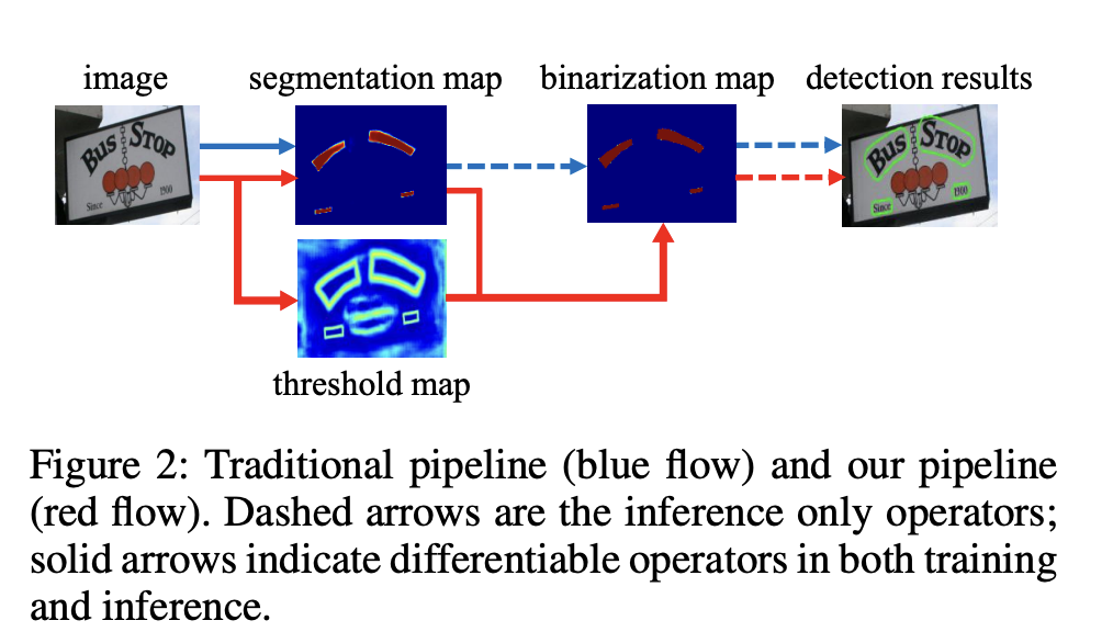
图1 DB模型与其他方法的区别

1.1 DBNet网络

1.1.1 网络结构

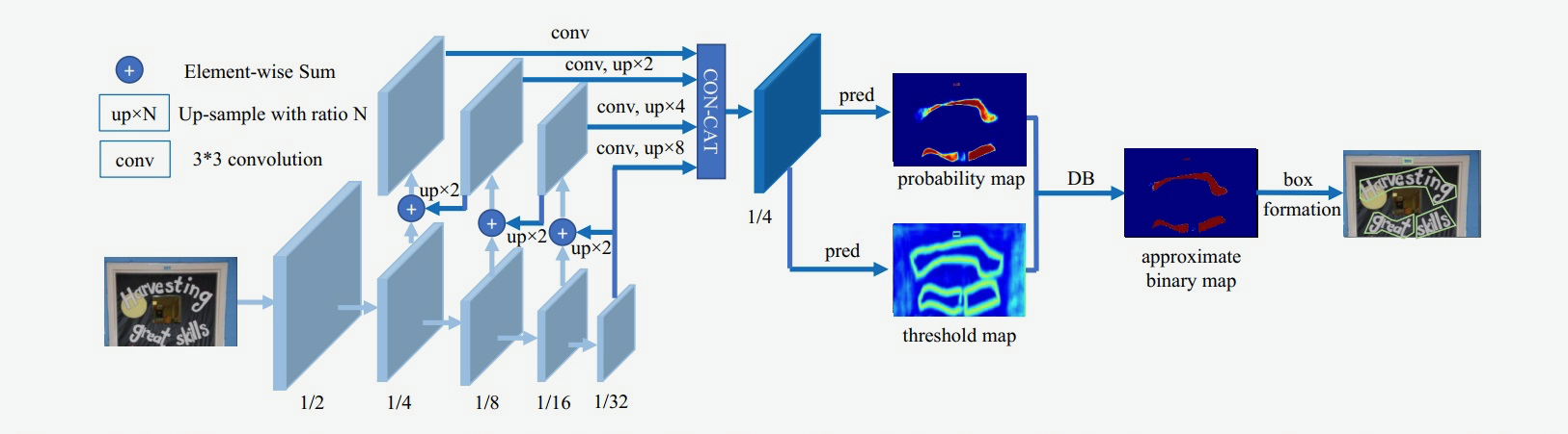
图2 DB模型网络结构示意图

DBNet的整个流程如下：
- 图像经过FPN网络结构，得到四个特征图，分别为1/4、1/8、1/16以及1/32大小；
- 将四个特征图分别上采样为1/4大小，然后concat，得到特征图F；
- 由F得到概率图probability map(P) 和阈值图threshold map(T)
- 通过P、T计算(计算公式后面介绍)得到近似二值图approximate binary map
对于每个网络，一定要区分训练和推理阶段的不同：
- 训练阶段：对P、T、B进行监督训练，P和B是用的相同的监督信号（label）；
- 推理阶段：通过P或B就可以得到文本框。

1.1.2 二值化操作

在传统的图像分割算法中，获取概率图后，会使用标准二值化（Standard Binarize）方法进行处理。
- 将低于阈值的像素点置0，高于阈值的像素点置1，公式如下：
  $B_{i,j}=\left\{ \begin{aligned} 1 , P_{i,j} >= t\\ 0 , otherwise. \end{aligned} \right.\\ 其中t为预先设定的固定阈值$
但是，标准的二值化方法是不可微的，导致网络无法端对端训练。
为了解决这个问题，DB算法提出了可微二值化（Differentiable Binarization，DB）。
- 可微二值化将标准二值化中的阶跃函数进行了近似，使用如下公式进行代替：
  $\hat{B} = \frac{1}{1 + e^{-k(P_{i,j}-T_{i,j})}}$
- 其中，P是上文中获取的概率图，T是上文中获取的阈值图，k是增益因子，在实验中，根据经验选取为50。
- 标准二值化和可微二值化的对比图如 下图3（a） 所示。可以看出，蓝色的DB曲线与黄色的SB曲线(标准二值化曲线)具有很高的相似度，并且DB曲线是可微分的，从而达到了二值化的目的。
- 由上文可以知道， $P_{i,j}$ 和 $T_{i,j}$ 是输入，所以可以将其看为输入，即 $P_{i,j}−T_{i,j}=x$ ，这样来看的话，这个函数其实就是一个带系数k的sigmoid函数。
那么，为什么可微分二值化会带来性能提升?
- DBNet性能提升的原因，我们可以通过梯度的反向传播进行解释
- 首先对于该任务的分割网络，每个像素点都是二分类，即文字区域(正样本为1)和非文字区域(负样本为0)，可以使用BCELoss
- 那么，当使用交叉熵损失时，正负样本的loss分别为 $l_+$ 和 $l_-$ ：
$l_+ = -log(\frac{1}{1 + e^{-k(P_{i,j}-T_{i,j})}})\\ l_- = -log(1-\frac{1}{1 + e^{-k(P_{i,j}-T_{i,j})}})$
- 对输入 $x$ 求偏导，则会得到下面式子：
$\frac{\delta{l_+}}{\delta{x}} = -kf(x)e^{-kx}\\ \frac{\delta{l_-}}{\delta{x}} = -kf(x)$
- 可以发现，增强因子会放大错误预测的梯度，从而优化模型得到更好的结果。
  - 图3（b） 中， $x < 0$ 的部分为正样本预测为负样本的情况，可以看到增益因子k将梯度进行了放大；
  - 图3（c） 中， $x > 0$ 的部分为负样本预测为正样本时，梯度同样也被放大了。

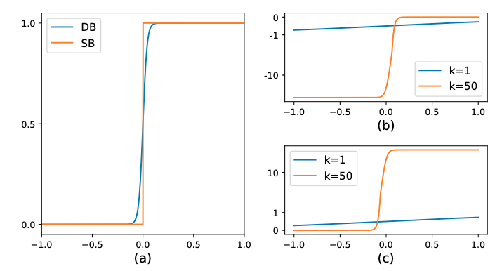
图3：DB算法示意图

1.2 标签生成

我们已经介绍了二值化操作，通过下面公式，我们很容易就得到了approximate binary map，接下来该计算损失函数，从而反向传播进行参数优化。

$\hat{B} = \frac{1}{1 + e^{-k(P_{i,j}-T_{i,j})}}\\ 其中，P是概率图，T是阈值图，k是增益因子，根据经验选取为50。\\ 概率图GT取值范围为0或1,文字区域为1，非文字区域为0\\ 阈值图GT取值范围为[0.3, 0.7],生成逻辑如下文$

概率图P和近似二值图 $\hat{B}$ 使用相同的标签，加上阈值图T的标签，所以需要生成两个标签。
要计算损失就需要标签，上文说到训练时，需要同时对P、T、B进行监督训练，P和B是用的相同的监督信号，T是作者加入的自适应阈值，那么为什么还需要对T进行监督呢？

1.2.1 概率图标签

下图上半部分是概率图P(也是近似二值图 $\hat{B}$ )的标签生成过程。
使用Vatti clipping算法，将原始的多边形文字区域G（红线区域）收缩到Gs（蓝线区域）
标签为：蓝线区域内为文字区域(标记为1)，蓝线区域外为非文字区域(标记为0)。
收缩的偏移量D的计算公式如下：

$D=\frac{A(1-r^2)}{L}\\ A是原始区域(红色框)的面积，L是原始区域的周长，r是收缩系数，依经验设置为r=0.4$

在这里插入图片描述

1.2.2 阈值图标签

阈值图的标签制作流程：

如上图下半部分所示，首先将原始的多边形文字区域G扩张到Gd（绿线区域），收缩偏移量D计算公式如上所示。
将收缩框Gs（蓝线）和扩张框Gd（绿线）之间的间隙视为文本区域的边界，计算这个间隙里每个像素点到原始图像边界G（红线）的归一化距离（最近线段的距离）。
计算完之后可以发现，扩张框Gd（绿线）上的像素点和收缩框Gs（蓝线）上的像素点的归一化距离的值是最大的，并且文字红线上的像素点的值最小，为0。呈现出以红线为基准，向Gs和Gd方向的值逐渐变大。
再对计算完的这些值进行归一化，也就是除以偏移量D，此时Gs（蓝线）和Gd（绿线）上的值变为1，再用1减去这些值。最后得到，红线上的值为1，Gs和Gd线上的值为0。呈现出以红线为基准，向Gs（蓝线）和Gd（绿线）方向的值逐渐变小。此时区域内的值取值范围为[0,1]。
最后，还需要进行一定的缩放，比如：将1缩放至0.7，将0缩放至0.3，此时区域内的值取值范围为[0.3,0.7]。

阈值图进行监督的原因：

下图的图c为没有监督的阈值图，虽然没有进行监督，但阈值图也会突出显示文本边界区域，这表明类似边界的阈值图有利于最终结果。
因此，作者在阈值图上应用了类似边界的监督，以提供更好的指导。下图中的图d为带监督的阈值图，显然效果更好了。

在这里插入图片描述

1.2.3 损失函数

损失函数为概率图的损失 $L_s$ 、二值化图的损失 $L_b$ 和阈值图的损失 $L_t$ 的和：
$L=L_s+\alpha L_b+\beta L_t\\ 其中\alpha和\beta分别设置为1和10\\$

$L_b$ 和 $L_t$ 都采用BCE Loss（二元交叉熵），为平衡正负样本的比例，使用OHEM进行困难样本挖掘，正样本:负样本=1:3

$L_b=L_s=\sum_{i\in S_l}y_ilogx_i + (1-y_i)log(1-x_i)\\ S_l表示使用OHEM进行采样，正负样本比例为1:3$

$L_t$ 使用Gd中预测值和标签值的 $L 1$ 距离

$L_t=\sum_{i\in R_d}|y_i^*-x_i^*| \\ R_d是Gd区域内的所有像素点，不仅仅是Gd和Gs区域内\\ y^*是阈值图的标签$

1.3 推理流程

在推理时，采用概率图或近似二值图便可计算出文本框，为了方便，作者选择了概率图，这样在推理时便可删掉阈值分支。文本框的形成可分为三个步骤：

1）使用固定阈值（0.2）对概率图（或近似二值图）进行二值化，得到二值图；
2）从二值图中得到连通区域（收缩文字区域）；
3）将收缩文字区域按Vatti clipping算法的偏移系数D’进行扩张得到最终文本框，D’的计算公式如下：

$D'=\frac{A'*r'}{L'}\\ 其中：A'、L'是收缩区域的面积、周长\\ r'设置为1.5（对应收缩比例r=0.4）$

推理阶段使用固定阈值的原因:

效率考虑：在推理阶段，为了获得更高的处理速度，通常会选择使用固定阈值对概率图进行二值化。这是因为自适应阈值图（T）的生成需要额外的计算资源，而在实际应用中，我们往往需要在保证检测精度的同时，尽可能提高处理速度。
简化后处理：在推理阶段，我们主要关注的是如何从概率图中提取出文本区域，并生成相应的边界框。使用固定阈值进行二值化后，可以通过简单的后处理步骤（如轮廓提取、边界框生成等）来得到最终的检测结果。这种方式不仅简单高效，而且能够满足大多数实际应用场景的需求。

2 DBNet在icdar15数据集上的微调(paddleocr)

我们这里使用百度开源的paddleocr来对CRNN模型有更深的认识：
- paddleocr地址：https://github.com/PaddlePaddle/PaddleOCR
- paddleocr中集成的算法列表：https://github.com/PaddlePaddle/PaddleOCR/blob/main/docs/algorithm/overview.md

# git拉取下来，解压
git clone https://gitee.com/paddlepaddle/PaddleOCR

# 然后进入PaddleOCR目录，安装PaddleOCR第三方依赖
pip install -r requirements.txt

我们在paddleocr/tests目录下，创建py文件进行下图的测试

在这里插入图片描述

百度将文字检测算法以及文字识别算法进行串联，构建了PP-OCR文字检测与识别系统。在实际使用过程中，检测出的文字方向可能不是我们期望的方向，最终导致文字识别错误，因此又在PP-OCR系统中引入了方向分类器。PP-OCR从工业界实用性角度出发，经历多次更新，论文如下：
- PP-OCR: https://arxiv.org/pdf/2009.09941
- PP-OCRv2: https://arxiv.org/pdf/2109.03144
- PP-OCRv3: https://arxiv.org/abs/2206.03001
- PP-OCRv4: 无论文

import cv2
import numpy as np
from paddleocr import PaddleOCR

ocr = PaddleOCR()

# 默认会下载官方训练好的模型，并将下载的模型放到用户目录下(我这里是：C:\\Users\\Undo/.paddleocr)
# rec=False表示：不使用识别模型进行识别，只执行文本检测
result = ocr.ocr(img=r'D:\python\py_works\paddleocr\tests\imgs\img_ppocr.png'
                 , det=True   # 文本检测器，默认算法为DBNet
                 , cls=True   # 方向分类器
                 , rec=False  # 文本识别，PP-OCRv2中默认为CRNN模型,不过从PP-OCRv3识别模块不再采用CRNN，更新为SVTR
                 )

print('=' * 50)
print(result)
print('=' * 50)

# 4. 可视化检测结果
image = cv2.imread(r'D:\python\py_works\paddleocr\tests\imgs\img_ppocr.png')
for box in result[0]:
    box = np.reshape(np.array(box), [-1, 1, 2]).astype(np.int64)
    image = cv2.polylines(np.array(image), [box], True, (255, 0, 0), 2)

# 画出读取的图片
cv2.imshow('image', image)
cv2.waitKey(0)
cv2.destroyAllWindows()

==================================================
[[[[75.0, 553.0], [448.0, 540.0], [449.0, 572.0], [77.0, 585.0]], [[18.0, 506.0], [514.0, 488.0], [516.0, 533.0], [20.0, 550.0]], [[187.0, 457.0], [398.0, 448.0], [400.0, 481.0], [188.0, 490.0]], [[40.0, 413.0], [483.0, 390.0], [485.0, 431.0], [42.0, 453.0]]]]
==================================================

在这里插入图片描述

2.1 DBNet网络的搭建

DBNet文本检测模型可以分为三个部分：

Backbone网络，负责提取图像的特征
Neck部分使用FPN网络，特征金字塔结构增强特征
Head网络，计算文本区域概率图

# paddleocr/configs/det/det_mv3_db.yml
Architecture:
  model_type: det
  algorithm: DB
  Transform:
  Backbone:
    name: MobileNetV3
    scale: 0.5
    model_name: large
  Neck:
    name: DBFPN
    out_channels: 256
  Head:
    name: DBHead
    k: 50

2.1.1 骨干网络

DB文本检测网络的Backbone部分采用的是图像分类网络，论文中使用了ResNet50，paddleocr/configs/det/det_mv3_db.yml中，采用MobileNetV3 large结构作为backbone。
DB的Backbone用于提取图像的多尺度特征，输入的形状为[640, 640]，backbone网络的输出有四个特征，其形状分别是：下采样4倍的C2[1, 16, 160, 160]，下采样8倍的C3[1, 24, 80, 80]，下采样16倍的C4[1, 56, 40, 40]，下采样16倍的C5[1, 480, 20, 20]。

# ppocr\modeling\backbones\det_mobilenet_v3.py

class MobileNetV3(nn.Layer):
    def __init__(
        self, in_channels=3, model_name="large", scale=0.5, disable_se=False, **kwargs
    ):
        """
        the MobilenetV3 backbone network for detection module.
        Args:
            params(dict): the super parameters for build network
        """
        super(MobileNetV3, self).__init__()

        self.disable_se = disable_se

        if model_name == "large":
            cfg = [
                # k, exp, c,  se,     nl,  s,
                [3, 16, 16, False, "relu", 1],
                [3, 64, 24, False, "relu", 2],
                [3, 72, 24, False, "relu", 1],        # C2 下采样4倍
                [5, 72, 40, True, "relu", 2],
                [5, 120, 40, True, "relu", 1],
                [5, 120, 40, True, "relu", 1],        # C3 下采样8倍
                [3, 240, 80, False, "hardswish", 2],
                [3, 200, 80, False, "hardswish", 1],
                [3, 184, 80, False, "hardswish", 1],
                [3, 184, 80, False, "hardswish", 1],
                [3, 480, 112, True, "hardswish", 1],
                [3, 672, 112, True, "hardswish", 1],  # C4 下采样16倍
                [5, 672, 160, True, "hardswish", 2],
                [5, 960, 160, True, "hardswish", 1],
                [5, 960, 160, True, "hardswish", 1],
            ]
            cls_ch_squeeze = 960
        elif model_name == "small":
            cfg = [
                # k, exp, c,  se,     nl,  s,
                [3, 16, 16, True, "relu", 2],
                [3, 72, 24, False, "relu", 2],
                [3, 88, 24, False, "relu", 1],
                [5, 96, 40, True, "hardswish", 2],
                [5, 240, 40, True, "hardswish", 1],
                [5, 240, 40, True, "hardswish", 1],
                [5, 120, 48, True, "hardswish", 1],
                [5, 144, 48, True, "hardswish", 1],
                [5, 288, 96, True, "hardswish", 2],
                [5, 576, 96, True, "hardswish", 1],
                [5, 576, 96, True, "hardswish", 1],
            ]
            cls_ch_squeeze = 576
        else:
            raise NotImplementedError(
                "mode[" + model_name + "_model] is not implemented!"
            )

        supported_scale = [0.35, 0.5, 0.75, 1.0, 1.25]
        assert (
            scale in supported_scale
        ), "supported scale are {} but input scale is {}".format(supported_scale, scale)
        inplanes = 16
        # conv1
        self.conv = ConvBNLayer(
            in_channels=in_channels,
            out_channels=make_divisible(inplanes * scale),
            kernel_size=3,
            stride=2,
            padding=1,
            groups=1,
            if_act=True,
            act="hardswish",
        )

        self.stages = []
        self.out_channels = []
        block_list = []
        i = 0
        inplanes = make_divisible(inplanes * scale)
        for k, exp, c, se, nl, s in cfg:
            se = se and not self.disable_se
            start_idx = 2 if model_name == "large" else 0
            if s == 2 and i > start_idx:
                self.out_channels.append(inplanes)
                self.stages.append(nn.Sequential(*block_list))
                block_list = []
            block_list.append(
                ResidualUnit(
                    in_channels=inplanes,
                    mid_channels=make_divisible(scale * exp),
                    out_channels=make_divisible(scale * c),
                    kernel_size=k,
                    stride=s,
                    use_se=se,
                    act=nl,
                )
            )
            inplanes = make_divisible(scale * c)
            i += 1
        # 最后一层卷积层
        block_list.append(
            ConvBNLayer(
                in_channels=inplanes,
                out_channels=make_divisible(scale * cls_ch_squeeze),
                kernel_size=1,
                stride=1,
                padding=0,
                groups=1,
                if_act=True,
                act="hardswish",
            )
        )  # C5 下采样32倍
        self.stages.append(nn.Sequential(*block_list))
        self.out_channels.append(make_divisible(scale * cls_ch_squeeze))
        for i, stage in enumerate(self.stages):
            self.add_sublayer(sublayer=stage, name="stage{}".format(i))

    def forward(self, x):
        x = self.conv(x)
        out_list = []
        # 将C2、C3、C4以及C5层的feature map进行保存
        # C2 shape = (bs, 16, 160, 160)
        # C3 shape = (bs, 24, 80, 80)
        # C4 shape = (bs, 56, 40, 40)
        # C5 shape = (bs, 480, 20, 20)
        for stage in self.stages:
            x = stage(x)
            out_list.append(x)
        return out_list

2.1.2 Neck部分

FPN的工作就是在检测前，先将多个尺度的特征图进行一次bottom-up的融合，这被证明是极其有效的特征融合方式，几乎成为了后来目标检测的标准模式之一；
DBNet中，也使用了FPN结构进行多尺度特征融合。

# paddleocr\ppocr\modeling\necks\db_fpn.py
class DBFPN(nn.Layer):
    def __init__(self, in_channels, out_channels, use_asf=False, **kwargs):
        super(DBFPN, self).__init__()
        self.out_channels = out_channels
        self.use_asf = use_asf
        weight_attr = paddle.nn.initializer.KaimingUniform()
        ......

    def forward(self, x):
        c2, c3, c4, c5 = x
        # 1、将c2, c3, c4, c5的通道数都调整为256
        in5 = self.in5_conv(c5)   # (bs, 256, 20, 20)
        in4 = self.in4_conv(c4)   # (bs, 256, 40, 40)
        in3 = self.in3_conv(c3)   # (bs, 256, 80, 80)
        in2 = self.in2_conv(c2)   # (bs, 256, 160, 160)
        # 2、通过FPN进行融合
        out4 = in4 + F.upsample(
            in5, scale_factor=2, mode="nearest", align_mode=1
        )  # 1/16
        out3 = in3 + F.upsample(
            out4, scale_factor=2, mode="nearest", align_mode=1
        )  # 1/8
        out2 = in2 + F.upsample(
            out3, scale_factor=2, mode="nearest", align_mode=1
        )  # 1/4
        # 3、通道数都调整为64(256/4)
        p5 = self.p5_conv(in5)     # (bs, 64, 20, 20)
        p4 = self.p4_conv(out4)    # (bs, 64, 40, 40)
        p3 = self.p3_conv(out3)    # (bs, 64, 80, 80)
        p2 = self.p2_conv(out2)    # (bs, 64, 160, 160)
        # 4、上采样到原图的1/4
        p5 = F.upsample(p5, scale_factor=8, mode="nearest", align_mode=1)
        p4 = F.upsample(p4, scale_factor=4, mode="nearest", align_mode=1)
        p3 = F.upsample(p3, scale_factor=2, mode="nearest", align_mode=1)
        # 在通道维度拼接 shape=(bs, 256, 160, 160)
        fuse = paddle.concat([p5, p4, p3, p2], axis=1)

        if self.use_asf is True:
            fuse = self.asf(fuse, [p5, p4, p3, p2])

        return fuse

2.1.3 Head网络

计算文本区域概率图，文本区域阈值图以及文本区域二值图

# ppocr\modeling\heads\det_db_head.py
class Head(nn.Layer):
    def __init__(self, in_channels, kernel_list=[3, 2, 2], **kwargs):
        super(Head, self).__init__()

        self.conv1 = nn.Conv2D(
            in_channels=in_channels,
            out_channels=in_channels // 4,
            kernel_size=kernel_list[0],
            padding=int(kernel_list[0] // 2),
            weight_attr=ParamAttr(),
            bias_attr=False,
        )
        self.conv_bn1 = nn.BatchNorm(
            num_channels=in_channels // 4,
            param_attr=ParamAttr(initializer=paddle.nn.initializer.Constant(value=1.0)),
            bias_attr=ParamAttr(initializer=paddle.nn.initializer.Constant(value=1e-4)),
            act="relu",
        )

        self.conv2 = nn.Conv2DTranspose(
            in_channels=in_channels // 4,
            out_channels=in_channels // 4,
            kernel_size=kernel_list[1],
            stride=2,
            weight_attr=ParamAttr(initializer=paddle.nn.initializer.KaimingUniform()),
            bias_attr=get_bias_attr(in_channels // 4),
        )
        self.conv_bn2 = nn.BatchNorm(
            num_channels=in_channels // 4,
            param_attr=ParamAttr(initializer=paddle.nn.initializer.Constant(value=1.0)),
            bias_attr=ParamAttr(initializer=paddle.nn.initializer.Constant(value=1e-4)),
            act="relu",
        )
        self.conv3 = nn.Conv2DTranspose(
            in_channels=in_channels // 4,
            out_channels=1,
            kernel_size=kernel_list[2],
            stride=2,
            weight_attr=ParamAttr(initializer=paddle.nn.initializer.KaimingUniform()),
            bias_attr=get_bias_attr(in_channels // 4),
        )

    def forward(self, x, return_f=False):
        # 1、通过3×3卷积降维:(bs, 256, 160, 160) -> (bs, 64, 160, 160)
        x = self.conv1(x)
        x = self.conv_bn1(x)
        # 2、通过转置卷积将feature map由原图的1/4大小映射到原图1/2: (bs, 64, 160, 160)-> (bs, 64, 320, 320)
        x = self.conv2(x)
        x = self.conv_bn2(x)
        if return_f is True:
            f = x
        # 3、通过转置卷积将feature map由原图的1/2大小映射到原图大小，并且输出维度为1: (bs, 64, 320, 320)-> (bs, 1, 640, 640)
        x = self.conv3(x)
        x = F.sigmoid(x)
        if return_f is True:
            return x, f
        return x

    
class DBHead(nn.Layer):
    """
    Differentiable Binarization (DB) for text detection:
        see https://arxiv.org/abs/1911.08947
    args:
        params(dict): super parameters for build DB network
    """

    def __init__(self, in_channels, k=50, **kwargs):
        super(DBHead, self).__init__()
        self.k = k
        self.binarize = Head(in_channels, **kwargs)
        self.thresh = Head(in_channels, **kwargs)

    def step_function(self, x, y):
        """
          可微二值化的实现，通过概率图和阈值图计算近似二值图
        """
        return paddle.reciprocal(1 + paddle.exp(-self.k * (x - y)))

    def forward(self, x, targets=None):
        # 1、获取概率图
        shrink_maps = self.binarize(x)       # (bs, 1, 640, 640)
        if not self.training:
            # 推理过程只需概率图
            return {"maps": shrink_maps}
        # 2、获取阈值图
        threshold_maps = self.thresh(x)      # (bs, 1, 640, 640)
        # 3、通过概率图和阈值图计算得到近似二值图
        binary_maps = self.step_function(shrink_maps, threshold_maps)  # (bs, 1, 640, 640)
        # 4、训练时，将概率图、阈值图以及近似二值图 按照通道进行拼接
        y = paddle.concat([shrink_maps, threshold_maps, binary_maps], axis=1)
        return {"maps": y}

2.2 数据集加载及模型训练

2.2.1 数据集的下载

提供一份处理过的icdar15数据集：
链接: https://pan.baidu.com/s/1ZYaS22cOv2FGIvOpd9FBdQ 提取码: rjbc

数据集应有如下文件结构：

text_localization 
  └─ icdar_c4_train_imgs/         icdar数据集的训练数据
  └─ ch4_test_images/             icdar数据集的测试数据
  └─ train_icdar2015_label.txt    icdar数据集的训练标注
  └─ test_icdar2015_label.txt     icdar数据集的测试标注

提供的标注文件格式为：

" 图像文件名                    json.dumps编码的图像标注信息"
ch4_test_images/img_61.jpg    [{"transcription": "MASA", "points": [[310, 104], [416, 141], [418, 216], [312, 179]], ...}]

json.dumps编码前的图像标注信息是包含多个字典的list，字典中的points表示文本框的四个点的坐标(x, y)，从左上角的点开始顺时针排列。 transcription中的字段表示当前文本框的文字，在文本检测任务中并不需要这个信息。如果您想在其他数据集上训练PaddleOCR，可以按照上述形式构建标注文件。
如果"transcription"字段的文字为’*‘或者’###‘，表示对应的标注可以被忽略掉，因此，如果没有文字标签，可以将transcription字段设置为空字符串。
下载完数据集后，我们复制一份paddleocr/configs/det/det_mv3_db.yml文件到paddleocr\tests\configs进行修改

2.2.2 模型的训练与预测

我这里不用命令行执行，在paddleocr\tests目录下创建一个py文件执行训练过程
通过下面的py文件，我们就可以愉快的查看源码了。

def train_det():
    from tools.train import program, set_seed, main
    # 配置文件的源地址地址： paddleocr/configs/det/det_mv3_db.yml
    config, device, logger, vdl_writer = program.preprocess(is_train=True)

    ###############修改配置（也可在yml文件中修改）##################
    # 加载预训练模型（模型下载地址如下）
    # https://paddleocr.bj.bcebos.com/pretrained/MobileNetV3_large_x0_5_pretrained.pdparams
    config["Global"]["pretrained_model"] = r"C:\Users\Undo\.paddleocr\whl\backbone\MobileNetV3_large_x0_5_pretrained"
    # 评估频率
    config["Global"]["eval_batch_step"] = [0, 200]
    # log的打印频率
    config["Global"]["print_batch_step"] = 10
    # 训练的epochs
    config["Global"]["epoch_num"] = 1
    # 随机种子
    seed = config["Global"]["seed"] if "seed" in config["Global"] else 1024
    set_seed(seed)

    ###############模型训练##################
    main(config, device, logger, vdl_writer, seed)

def infer_det():
    # 加载自己训练的模型
    from tools.infer_det import main, program

    config, device, logger, vdl_writer = program.preprocess()
    config["Global"]["use_gpu"] = False
    config["Global"]["infer_img"] = r"D:\python\py_works\paddleocr\doc\imgs_en\img_12.jpg"
    config["Global"]["checkpoints"] = r"D:\python\py_works\paddleocr\tests\output\db_mv3\best_accuracy"
    # 这里加了add_config这个参数，源码中没有
    main(add_config=(config, device, logger, vdl_writer))


if __name__ == '__main__':
    train_det()
    # infer_det()

main方法中定义了训练的脚本

# paddleocr/tools/train.py
def main(config, device, logger, vdl_writer, seed):
    # init dist environment
    if config["Global"]["distributed"]:
        dist.init_parallel_env()

    global_config = config["Global"]

    # build dataloader
    set_signal_handlers()
    # 1、创建dataloader
    train_dataloader = build_dataloader(config, "Train", device, logger, seed)

    ......
    if config["Eval"]:
        valid_dataloader = build_dataloader(config, "Eval", device, logger, seed)
    else:
        valid_dataloader = None
    step_pre_epoch = len(train_dataloader)

    # 2、后处理程序
    # build post process
    post_process_class = build_post_process(config["PostProcess"], global_config)

    # 3、模型构建
    # build model
    .....
    model = build_model(config["Architecture"])

    use_sync_bn = config["Global"].get("use_sync_bn", False)
    if use_sync_bn:
        model = paddle.nn.SyncBatchNorm.convert_sync_batchnorm(model)
        logger.info("convert_sync_batchnorm")

    model = apply_to_static(model, config, logger)

    # 4、构建损失函数
    # build loss
    loss_class = build_loss(config["Loss"])

    # 5、构建优化器
    # build optim
    optimizer, lr_scheduler = build_optimizer(
        config["Optimizer"],
        epochs=config["Global"]["epoch_num"],
        step_each_epoch=len(train_dataloader),
        model=model,
    )

    # 6、创建评估函数
    # build metric
    eval_class = build_metric(config["Metric"])
    ......

    # 7、加载预训练模型
    # load pretrain model
    pre_best_model_dict = load_model(
        config, model, optimizer, config["Architecture"]["model_type"]
    )

    if config["Global"]["distributed"]:
        model = paddle.DataParallel(model)

    # 8、模型训练
    # start train
    program.train(
        config,
        train_dataloader,
        valid_dataloader,
        device,
        model,
        loss_class,
        optimizer,
        lr_scheduler,
        post_process_class,
        eval_class,
        pre_best_model_dict,
        logger,
        step_pre_epoch,
        vdl_writer,
        scaler,
        amp_level,
        amp_custom_black_list,
        amp_custom_white_list,
        amp_dtype,
    )

2.2.3 数据预处理

数据预处理共包括如下方法：

图像解码：将图像转为Numpy格式；
标签解码：解析txt文件中的标签信息，并按统一格式进行保存；
基础数据增广：包括：随机水平翻转、随机旋转，随机缩放，随机裁剪等；
获取阈值图标签：使用扩张的方式获取算法训练需要的阈值图标签；
获取概率图标签：使用收缩的方式获取算法训练需要的概率图标签；
归一化：通过规范化手段，把神经网络每层中任意神经元的输入值分布改变成均值为0，方差为1的标准正太分布，使得最优解的寻优过程明显会变得平缓，训练过程更容易收敛；
通道变换：图像的数据格式为[H, W, C]（即高度、宽度和通道数），而神经网络使用的训练数据的格式为[C, H, W]，因此需要对图像数据重新排列，例如[224, 224, 3]变为[3, 224, 224]；

这里我们主要看下：获取阈值图标签以及获取概率图标签的实现, 原理可以参考：1.2章节

Train:
  dataset:
    name: SimpleDataSet
    data_dir: D:\python\datas\cv\icdar2015\text_localization\
    label_file_list:
      - D:\python\datas\cv\icdar2015\text_localization\train_icdar2015_label.txt
    ratio_list: [1.0]
    transforms:
      - DecodeImage: # load image
          img_mode: BGR
          channel_first: False
      - DetLabelEncode: # Class handling label
      - IaaAugment:
          augmenter_args:
            - { 'type': Fliplr, 'args': { 'p': 0.5 } }              # 随机水平翻转
            - { 'type': Affine, 'args': { 'rotate': [-10, 10] } }   # 随机旋转
            - { 'type': Resize, 'args': { 'size': [0.5, 3] } }      # 随机缩放
      - EastRandomCropData:
          size: [640, 640]   # 随机裁剪
          max_tries: 50
          keep_ratio: true
      - MakeBorderMap:       # 阈值图标签的生成 ppocr/data/imaug/make_border_map.py
          shrink_ratio: 0.4
          thresh_min: 0.3
          thresh_max: 0.7
      - MakeShrinkMap:     # 概率图标签的生成  ppocr/data/imaug/make_shrink_map.py
          shrink_ratio: 0.4
          min_text_size: 8
      - NormalizeImage:   # 通过规范化手段，把神经网络每层中任意神经元的输入值分布改变成均值为0，方差为1的标准正太分布，使得最优解的寻优过程明显会变得平缓，训练过程更容易收敛
          scale: 1./255.
          mean: [0.485, 0.456, 0.406]
          std: [0.229, 0.224, 0.225]
          order: 'hwc'
      - ToCHWImage: # 图像的数据格式为[H, W, C]（即高度、宽度和通道数），而神经网络使用的训练数据的格式为[C, H, W]，因此需要对图像数据重新排列
      - KeepKeys:
          keep_keys: ['image', 'threshold_map', 'threshold_mask', 'shrink_map', 'shrink_mask'] # the order of the dataloader list
  loader:
    shuffle: True
    drop_last: False
    batch_size_per_card: 4
    num_workers: 0
    use_shared_memory: False

Eval:
  dataset:
    name: SimpleDataSet
    data_dir: D:\python\datas\cv\icdar2015\text_localization\
    label_file_list:
      - D:\python\datas\cv\icdar2015\text_localization\test_icdar2015_label.txt
    transforms:
      - DecodeImage: # load image
          img_mode: BGR
          channel_first: False
      - DetLabelEncode: # Class handling label
      - DetResizeForTest:
          image_shape: [736, 1280]
      - NormalizeImage:
          scale: 1./255.
          mean: [0.485, 0.456, 0.406]
          std: [0.229, 0.224, 0.225]
          order: 'hwc'
      - ToCHWImage:
      - KeepKeys:
          keep_keys: ['image', 'shape', 'polys', 'ignore_tags']
  loader:
    shuffle: False
    drop_last: False
    batch_size_per_card: 1 # must be 1
    num_workers: 0
    use_shared_memory: True

获取概率图标签

# paddleocr\ppocr\data\imaug\make_shrink_map.py
class MakeShrinkMap(object):
    r"""
    Making binary mask from detection data with ICDAR format.
    Typically following the process of class `MakeICDARData`.
    """

    def __init__(self, min_text_size=8, shrink_ratio=0.4, **kwargs):
        self.min_text_size = min_text_size
        self.shrink_ratio = shrink_ratio
        if "total_epoch" in kwargs and "epoch" in kwargs and kwargs["epoch"] != "None":
            self.shrink_ratio = self.shrink_ratio + 0.2 * kwargs["epoch"] / float(
                kwargs["total_epoch"]
            )

    def __call__(self, data):
        image = data["image"]             # (640, 640, 3), 一张图片的shape
        text_polys = data["polys"]        # (4, 4, 2), 一张图片有4个文字块，每个文字块bbox坐标shape为(4, 2)
        ignore_tags = data["ignore_tags"] # [True, False, True, True]， True表示此标注无效

        h, w = image.shape[:2]
        # 1. 校验文本检测标签
        text_polys, ignore_tags = self.validate_polygons(text_polys, ignore_tags, h, w)
        gt = np.zeros((h, w), dtype=np.float32)
        mask = np.ones((h, w), dtype=np.float32)

        # 2. 根据文本检测框计算文本区域概率图
        for i in range(len(text_polys)):
            polygon = text_polys[i]
            height = max(polygon[:, 1]) - min(polygon[:, 1])
            width = max(polygon[:, 0]) - min(polygon[:, 0])
            if ignore_tags[i] or min(height, width) < self.min_text_size:
                # 如果该文本块无效或其尺寸小于最小文本尺寸 (self.min_text_size)，则将该区域在mask中设为0，并标记为无效
                cv2.fillPoly(mask, polygon.astype(np.int32)[np.newaxis, :, :], 0)
                ignore_tags[i] = True
            else:
                # 对有效的文本块，使用shapely库的Polygon创建多边形对象，并使用pyclipper进行后续的收缩操作
                polygon_shape = Polygon(polygon)
                subject = [tuple(l) for l in polygon]
                padding = pyclipper.PyclipperOffset()
                # 将多边形的顶点（即subject）添加到padding中
                # JT_ROUND：表示在进行偏移时，角落会被圆滑处理；ET_CLOSEDPOLYGON：表示这是一个封闭的多边形
                padding.AddPath(subject, pyclipper.JT_ROUND, pyclipper.ET_CLOSEDPOLYGON)
                shrinked = []

                # Increase the shrink ratio every time we get multiple polygon returned back
                # 生成多个收缩系数，这些系数用于缩小多边形的边界，如: [0.4, 0.8]
                possible_ratios = np.arange(self.shrink_ratio, 1, self.shrink_ratio)
                np.append(possible_ratios, 1)
                # print(possible_ratios)
                # 对每个收缩系数，计算收缩的偏移量，然后尝试收缩多边形。若成功收缩得到一个多边形，则退出循环
                for ratio in possible_ratios:
                    # print(f"Change shrink ratio to {ratio}")
                    # 计算收缩的偏移量
                    distance = (
                        polygon_shape.area         # 文字块，即原始区域的面积
                        * (1 - np.power(ratio, 2)) # ratio为收缩系数
                        / polygon_shape.length     # 文字块，即原始区域的周长
                    )
                    # 参数 -distance表示收缩的距离。负值表示将多边形向内收缩
                    # 如果distance合适且收缩成功，通常会返回一个或多个新的多边形。
                    shrinked = padding.Execute(-distance)
                    # 在某些情况下，收缩操作可能会产生多个多边形，尤其是在原始多边形形状复杂或者收缩比例不合适的情况下
                    # 因此，这里一旦找到一个有效的收缩结果，使用break跳出循环，避免继续使用其他收缩比例，这样可以提高效率，并确保结果的简洁性
                    if len(shrinked) == 1:
                        break

                if shrinked == []:
                    # 如果没有成功收缩，标记该多边形为无效
                    cv2.fillPoly(mask, polygon.astype(np.int32)[np.newaxis, :, :], 0)
                    ignore_tags[i] = True
                    continue

                for each_shirnk in shrinked:
                    # 如果成功收缩，则更新gt概率图，将收缩后的多边形区域设为1，表示该区域包含文本
                    shirnk = np.array(each_shirnk).reshape(-1, 2)
                    cv2.fillPoly(gt, [shirnk.astype(np.int32)], 1)

        # 将生成的概率图(gt)和掩码(mask)存入data字典，并返回
        data["shrink_map"] = gt
        data["shrink_mask"] = mask
        return data
    
        ......

获取阈值图标签

# paddleocr\ppocr\data\imaug\make_border_map.py
class MakeBorderMap(object):
    def __init__(self, shrink_ratio=0.4, thresh_min=0.3, thresh_max=0.7, **kwargs):
        self.shrink_ratio = shrink_ratio
        self.thresh_min = thresh_min
        self.thresh_max = thresh_max
        if "total_epoch" in kwargs and "epoch" in kwargs and kwargs["epoch"] != "None":
            self.shrink_ratio = self.shrink_ratio + 0.2 * kwargs["epoch"] / float(
                kwargs["total_epoch"]
            )

    def __call__(self, data):
        img = data["image"]               # (640, 640, 3), 一张图片的shape
        text_polys = data["polys"]        # (4, 4, 2), 一张图片有4个文字块，每个文字块bbox坐标shape为(4, 2)
        ignore_tags = data["ignore_tags"] # [True, False, True, True]， True表示此标注无效

        # 1. 生成空模版
        canvas = np.zeros(img.shape[:2], dtype=np.float32)
        mask = np.zeros(img.shape[:2], dtype=np.float32)

        for i in range(len(text_polys)):
            if ignore_tags[i]:
                continue
            # 2. draw_border_map函数根据解码后的box信息计算阈值图标签
            self.draw_border_map(text_polys[i], canvas, mask=mask)
        # 将canvas归一化到一个指定的阈值范围(thresh_min=0.3和thresh_max=0.7)
        canvas = canvas * (self.thresh_max - self.thresh_min) + self.thresh_min

        data["threshold_map"] = canvas
        data["threshold_mask"] = mask
        return data

    def draw_border_map(self, polygon, canvas, mask):
        """
        polygon: 输入的多边形顶点，形状为(n, 2)，其中n是顶点数量，每个顶点由两个坐标(x, y) 表示。
        canvas: 用于存储最终生成的阈值图的画布（2D数组）。
        mask: 用于存储掩码的画布（2D数组）。
        """
        polygon = np.array(polygon)
        assert polygon.ndim == 2
        assert polygon.shape[1] == 2

        polygon_shape = Polygon(polygon)
        if polygon_shape.area <= 0:
            return
        # 计算收缩后的距离 distance
        distance = (
            polygon_shape.area
            * (1 - np.power(self.shrink_ratio, 2))
            / polygon_shape.length
        )
        subject = [tuple(l) for l in polygon]
        padding = pyclipper.PyclipperOffset()
        padding.AddPath(subject, pyclipper.JT_ROUND, pyclipper.ET_CLOSEDPOLYGON)
        # 调用Execute(distance)来收缩多边形，返回的结果是收缩后的多边形
        # 需要注意的是，该方法返回一个列表，通常只需要第一个元素
        padded_polygon = np.array(padding.Execute(distance)[0])
        # 在掩码上填充收缩后的多边形区域，值设置为 1.0，表示该区域有效
        cv2.fillPoly(mask, [padded_polygon.astype(np.int32)], 1.0)

        # 计算收缩后多边形的最小和最大x, y坐标，从而确定其边界框（bounding box）的位置和大小
        xmin = padded_polygon[:, 0].min()
        xmax = padded_polygon[:, 0].max()
        ymin = padded_polygon[:, 1].min()
        ymax = padded_polygon[:, 1].max()
        width = xmax - xmin + 1
        height = ymax - ymin + 1

        # 将多边形的坐标调整到边界框内，以便后续计算距离图
        polygon[:, 0] = polygon[:, 0] - xmin
        polygon[:, 1] = polygon[:, 1] - ymin
        # 生成网格坐标: 创建一个宽度和高度的网格，xs和ys分别表示每个点的x和y坐标
        xs = np.broadcast_to(
            np.linspace(0, width - 1, num=width).reshape(1, width), (height, width)
        )
        ys = np.broadcast_to(
            np.linspace(0, height - 1, num=height).reshape(height, 1), (height, width)
        )

        distance_map = np.zeros((polygon.shape[0], height, width), dtype=np.float32)
        # 遍历多边形的每条边，调用_distance方法计算网格上每个点到边的距离，并将其归一化到[0, 1]范围内
        for i in range(polygon.shape[0]):
            j = (i + 1) % polygon.shape[0]
            absolute_distance = self._distance(xs, ys, polygon[i], polygon[j])
            distance_map[i] = np.clip(absolute_distance / distance, 0, 1)
        # 将所有边的距离图合并成一个单一的距离图，表示每个点到最近边的距离
        distance_map = distance_map.min(axis=0)

        xmin_valid = min(max(0, xmin), canvas.shape[1] - 1)
        xmax_valid = min(max(0, xmax), canvas.shape[1] - 1)
        ymin_valid = min(max(0, ymin), canvas.shape[0] - 1)
        ymax_valid = min(max(0, ymax), canvas.shape[0] - 1)

        #  np.fmax用于逐元素比较两个数组或数值，并返回它们的最大值
        # 使用np.fmax将计算出的距离图与现有的canvas进行比较，更新画布的值
        # 这里的更新是通过将距离值反转（1 - distance_map）来实现的，表示距离较近的区域将具有较高的值（接近1）
        canvas[ymin_valid : ymax_valid + 1, xmin_valid : xmax_valid + 1] = np.fmax(
            1
            - distance_map[
                ymin_valid - ymin : ymax_valid - ymax + height,
                xmin_valid - xmin : xmax_valid - xmax + width,
            ],
            canvas[ymin_valid : ymax_valid + 1, xmin_valid : xmax_valid + 1],
        )

2.2.4 构建数据读取器

采用PaddlePaddle中的Dataset构建数据读取器

# ppocr/data/simple_dataset.py
def transform(data, ops=None):
    """ transform """
    if ops is None:
        ops = []
    for op in ops:
        data = op(data)
        if data is None:
            return None
    return data


def create_operators(op_param_list, global_config=None):
    """
    create operators based on the config
    Args:
        params(list): a dict list, used to create some operators
    """
    assert isinstance(op_param_list, list), ('operator config should be a list')
    ops = []
    for operator in op_param_list:
        assert isinstance(operator,
                          dict) and len(operator) == 1, "yaml format error"
        op_name = list(operator)[0]
        param = {} if operator[op_name] is None else operator[op_name]
        if global_config is not None:
            param.update(global_config)
        op = eval(op_name)(**param)
        ops.append(op)
    return ops

    
class SimpleDataSet(Dataset):
    def __init__(self, mode, label_file, data_dir, seed=None):
        super(SimpleDataSet, self).__init__()
        # 标注文件中，使用'\t'作为分隔符区分图片名称与标签
        self.delimiter = '\t'
        # 数据集路径
        self.data_dir = data_dir
        # 随机数种子
        self.seed = seed
        # 获取所有数据，以列表形式返回
        self.data_lines = self.get_image_info_list(label_file)
        # 新建列表存放数据索引
        self.data_idx_order_list = list(range(len(self.data_lines)))
        self.mode = mode
        # 如果是训练过程，将数据集进行随机打乱
        if self.mode.lower() == "train":
            self.shuffle_data_random()

    def get_image_info_list(self, label_file):
        # 获取标签文件中的所有数据
        with open(label_file, "rb") as f:
            lines = f.readlines()
        return lines

    def shuffle_data_random(self):
        #随机打乱数据
        random.seed(self.seed)
        random.shuffle(self.data_lines)
        return

    def __getitem__(self, idx):
        # 1. 获取索引为idx的数据
        file_idx = self.data_idx_order_list[idx]
        data_line = self.data_lines[file_idx]
        try:
            # 2. 获取图片名称以及标签
            data_line = data_line.decode('utf-8')
            substr = data_line.strip("\n").split(self.delimiter)
            file_name = substr[0]
            label = substr[1]
            # 3. 获取图片路径
            img_path = os.path.join(self.data_dir, file_name)
            data = {'img_path': img_path, 'label': label}
            if not os.path.exists(img_path):
                raise Exception("{} does not exist!".format(img_path))
            # 4. 读取图片并进行预处理
            with open(data['img_path'], 'rb') as f:
                img = f.read()
                data['image'] = img

            # 5. 完成数据增强操作
            outs = transform(data, self.mode.lower())

        # 6. 如果当前数据读取失败，重新随机读取一个新数据
        except Exception as e:
            outs = None
        if outs is None:
            return self.__getitem__(np.random.randint(self.__len__()))
        return outs

    def __len__(self):
        # 返回数据集的大小
        return len(self.data_idx_order_list)

通过build_dataloader加载数据集

# paddleocr/ppocr/data/__init__.py
def build_dataloader(config, mode, device, logger, seed=None):
    config = copy.deepcopy(config)

    support_dict = [
        "SimpleDataSet", # 配置文件中为SimpleDataSet
        "LMDBDataSet",
        "PGDataSet",
        "PubTabDataSet",
        "LMDBDataSetSR",
        "LMDBDataSetTableMaster",
        "MultiScaleDataSet",
        "TextDetDataset",
        "TextRecDataset",
        "MSTextRecDataset",
        "PubTabTableRecDataset",
        "KieDataset",
        "LaTeXOCRDataSet",
    ]
    module_name = config[mode]["dataset"]["name"]
    assert module_name in support_dict, Exception(
        "DataSet only support {}".format(support_dict)
    )
    assert mode in ["Train", "Eval", "Test"], "Mode should be Train, Eval or Test."
    # 1、创建dataset
    dataset = eval(module_name)(config, mode, logger, seed)
    ......
    # 2、创建data_loader
    data_loader = DataLoader(
        dataset=dataset,
        batch_sampler=batch_sampler,
        places=device,
        num_workers=num_workers,
        return_list=True,
        use_shared_memory=use_shared_memory,
        collate_fn=collate_fn,
    )

    return data_loader

2.2.5 损失函数的构建

由于训练阶段获取了3个预测图，所以在损失函数中，也需要结合这3个预测图与它们对应的真实标签分别构建3部分损失函数。总的损失函数的公式定义如下:

$L_b + \alpha \times L_s + \beta \times L_t$

其中， $L$ 为总的损失， $L_s$ 为概率图损失，在本实验中使用了带 OHEM（online hard example mining）的 Dice 损失， $L_t$ 为阈值图损失，在本实验中使用了预测值和标签间的 $L_1$ 距离， $L_b$ 为文本二值图的损失函数。 $\alpha$ 和 $\beta$ 为权重系数，本实验中分别将其设为5和10。

三个loss $L_b$ ， $L_s$ ， $L_t$ 分别是Dice Loss、Dice Loss(OHEM)、MaskL1 Loss，接下来分别定义这3个部分：

Dice Loss是比较预测的文本二值图和标签之间的相似度，常用于二值图像分割，公式如下：

$dice\_loss = 1 - \frac{2 \times intersection\_area}{total\_area}$

Dice Loss(OHEM)是采用带OHEM的Dice Loss，目的是为了改善正负样本不均衡的问题。OHEM为一种特殊的自动采样方式，可以自动的选择难样本进行loss的计算，从而提升模型的训练效果。这里将正负样本的采样比率设为1:3。
MaskL1 Loss是计算预测的文本阈值图和标签间的 $L_1$ 距离。

# paddleocr\ppocr\losses\det_db_loss.py
class DBLoss(nn.Layer):
    """
    Differentiable Binarization (DB) Loss Function
    args:
        param (dict): the super paramter for DB Loss
    """

    def __init__(
        self,
        balance_loss=True,
        main_loss_type="DiceLoss",
        alpha=5,
        beta=10,
        ohem_ratio=3,
        eps=1e-6,
        **kwargs,
    ):
        super(DBLoss, self).__init__()
        self.alpha = alpha
        self.beta = beta
        self.dice_loss = DiceLoss(eps=eps)
        self.l1_loss = MaskL1Loss(eps=eps)
        self.bce_loss = BalanceLoss(
            balance_loss=balance_loss,
            main_loss_type=main_loss_type,
            negative_ratio=ohem_ratio,
        )

    def forward(self, predicts, labels):
        # 1、获取阈值图标签以及概率图标签(也是二值图标签)
        (
            label_threshold_map,
            label_threshold_mask,
            label_shrink_map,
            label_shrink_mask,
        ) = labels[1:]
        # 2、获取预测的概率图、阈值图以及近似二值图
        predict_maps = predicts["maps"]
        shrink_maps = predict_maps[:, 0, :, :]
        threshold_maps = predict_maps[:, 1, :, :]
        binary_maps = predict_maps[:, 2, :, :]

        # 概率图计算bce_loss
        loss_shrink_maps = self.bce_loss(
            shrink_maps, label_shrink_map, label_shrink_mask
        )
        # 阈值图计算l1_loss
        loss_threshold_maps = self.l1_loss(
            threshold_maps, label_threshold_map, label_threshold_mask
        )
        # 近似二值图计算dice_loss
        # dice_loss特别适用于像素级别的二分类或多分类任务
        loss_binary_maps = self.dice_loss(
            binary_maps, label_shrink_map, label_shrink_mask
        )
        loss_shrink_maps = self.alpha * loss_shrink_maps
        loss_threshold_maps = self.beta * loss_threshold_maps
        # CBN loss
        if "distance_maps" in predicts.keys():
            distance_maps = predicts["distance_maps"]
            cbn_maps = predicts["cbn_maps"]
            cbn_loss = self.bce_loss(
                cbn_maps[:, 0, :, :], label_shrink_map, label_shrink_mask
            )
        else:
            dis_loss = paddle.to_tensor([0.0])
            cbn_loss = paddle.to_tensor([0.0])

        loss_all = loss_shrink_maps + loss_threshold_maps + loss_binary_maps
        losses = {
            "loss": loss_all + cbn_loss,
            "loss_shrink_maps": loss_shrink_maps,
            "loss_threshold_maps": loss_threshold_maps,
            "loss_binary_maps": loss_binary_maps,
            "loss_cbn": cbn_loss,
        }
        return losses

2.2.6 预测过程中的后处理程序

原理可以参考：1.3章节

PostProcess:
  name: DBPostProcess
  thresh: 0.3
  box_thresh: 0.6
  max_candidates: 1000
  unclip_ratio: 1.5

class DBPostProcess(object):
    """
    The post process for Differentiable Binarization (DB).

    DB后处理有四个参数，分别是：
        thresh: DBPostProcess中分割图进行二值化的阈值，默认值为0.3
        box_thresh: DBPostProcess中对输出框进行过滤的阈值，低于此阈值的框不会输出
        unclip_ratio: DBPostProcess中对文本框进行放大的比例
        max_candidates: DBPostProcess中输出的最大文本框数量，默认1000
    """

    def __init__(
        self,
        thresh=0.3,
        box_thresh=0.7,
        max_candidates=1000,
        unclip_ratio=2.0,
        use_dilation=False,
        score_mode="fast",
        box_type="quad",
        **kwargs,
    ):
        self.thresh = thresh
        self.box_thresh = box_thresh
        self.max_candidates = max_candidates
        self.unclip_ratio = unclip_ratio
        self.min_size = 3
        self.score_mode = score_mode
        self.box_type = box_type
        assert score_mode in [
            "slow",
            "fast",
        ], "Score mode must be in [slow, fast] but got: {}".format(score_mode)

        self.dilation_kernel = None if not use_dilation else np.array([[1, 1], [1, 1]])

       

    def boxes_from_bitmap(self, pred, _bitmap, dest_width, dest_height):
        """
        _bitmap: single map with shape (1, H, W),
                whose values are binarized as {0, 1}

        输入: pred_shape = (736, 1280), mask_shape = (736, 1280), src_w=1680, src_h=1048
        结果： boxes_shape = (10, 4, 2), scores_len = 10
        """
        bitmap = _bitmap
        height, width = bitmap.shape
        # cv2.findContours函数可以在二值图像中查找轮廓, 该函数可以检测图像中的白色或黑色区域，并返回这些区域的边界
        outs = cv2.findContours(
            (bitmap * 255).astype(np.uint8), cv2.RETR_LIST, cv2.CHAIN_APPROX_SIMPLE
        )
        if len(outs) == 3:
            img, contours, _ = outs[0], outs[1], outs[2]
        elif len(outs) == 2:
            # contours：一个Python列表，其中每个元素都是一个轮廓，轮廓是一个点集（通常是numpy数组的形式）
            contours, _ = outs[0], outs[1]

        # 输出的最大文本框数量，默认1000
        num_contours = min(len(contours), self.max_candidates)

        boxes = []
        scores = []
        for index in range(num_contours):
            # contour_shape = (4, 1, 2)
            contour = contours[index]
            # 返回轮廓最小外接矩形的四个顶点坐标以及它的最小边长
            points, sside = self.get_mini_boxes(contour)
            if sside < self.min_size:     # 最小边长阈值为3
                continue
            points = np.array(points)
            if self.score_mode == "fast":
                # 通过计算边界框内部像素的平均值获取 score
                score = self.box_score_fast(pred, points.reshape(-1, 2))
            else:
                score = self.box_score_slow(pred, contour)
            if self.box_thresh > score:   # 对输出框进行过滤的阈值，低于此阈值的框不会输出，默认为0.6
                continue

            # 将收缩文字区域按Vatti clipping算法的偏移系数D'进行扩张得到最终文本框
            box = self.unclip(points, self.unclip_ratio)
            if len(box) > 1:
                continue
            box = np.array(box).reshape(-1, 1, 2)
            # 返回扩张后轮廓最小外接矩形的四个顶点坐标以及它的最小边长
            box, sside = self.get_mini_boxes(box)
            if sside < self.min_size + 2:
                continue
            box = np.array(box)

            # 从原始尺寸转换为目标尺寸, 并确保边界框不会超出目标图像边界
            box[:, 0] = np.clip(np.round(box[:, 0] / width * dest_width), 0, dest_width)
            box[:, 1] = np.clip(
                np.round(box[:, 1] / height * dest_height), 0, dest_height
            )
            boxes.append(box.astype("int32"))
            scores.append(score)
        return np.array(boxes, dtype="int32"), scores

    def unclip(self, box, unclip_ratio):
        poly = Polygon(box)
        # 偏移系数D' = A' * r' / L', 其中：A'为收缩区域的面积，L'为收缩区域的周长， r'默认设置为1.5
        distance = poly.area * unclip_ratio / poly.length
        offset = pyclipper.PyclipperOffset()
        offset.AddPath(box, pyclipper.JT_ROUND, pyclipper.ET_CLOSEDPOLYGON)
        expanded = offset.Execute(distance)
        return expanded

    def get_mini_boxes(self, contour):
        """
            从给定的轮廓(contour)中计算出一个最小外接矩形，并返回这个矩形的四个顶点坐标以及它的最小边长
        """
        # 1、计算给定轮廓的最小外接矩形
        # cv2.minAreaRect函数返回一个Box2D对象，包含矩形的中心坐标、宽高（宽度和高度可能以任意顺序给出）以及旋转角度
        bounding_box = cv2.minAreaRect(contour)

        # 2、获取矩形的四个顶点
        # cv2.boxPoints函数根据bounding_box计算出矩形的四个顶点坐标，例如：
        # array([[797.00006, 578.     ],
        #        [798.00006, 577.     ],
        #        [799.00006, 578.     ],
        #        [798.00006, 579.     ]], dtype=float32)
        # 然后，将这些顶点坐标转换为一个列表，并使用 sorted 函数对这些点进行排序。
        # 排序的依据是顶点的x坐标（即顶点的水平位置），这样可以确保顶点按照它们在矩形上的顺序排列
        # 转换顺序后：
        # [   [797.00006, 578.     ],
        #     [798.00006, 577.     ],
        #     [798.00006, 579.     ],
        #     [799.00006, 578.     ]]
        points = sorted(list(cv2.boxPoints(bounding_box)), key=lambda x: x[0])

        # 3、确定矩形的四个顶点顺序
        # 通过比较顶点的y坐标（即顶点的垂直位置）来确定矩形的左上角、右上角、右下角和左下角的顶点顺序
        # 由于最小外接矩形可能是倾斜的，简单的上下左右判断不足以确定顶点顺序，因此需要根据y坐标的比较来确定
        index_1, index_2, index_3, index_4 = 0, 1, 2, 3
        if points[1][1] > points[0][1]:
            index_1 = 0
            index_4 = 1
        else:
            index_1 = 1
            index_4 = 0
        if points[3][1] > points[2][1]:
            index_2 = 2
            index_3 = 3
        else:
            index_2 = 3
            index_3 = 2
        # ndex_1和index_4对应于矩形的左边界的两个顶点，index_2和index_3对应于右边界的两个顶点
        # 最终的box信息：
        #    [[798.00006, 577.],
        #     [799.00006, 578.],
        #     [798.00006, 579.],
        #     [797.00006, 578.]]
        box = [points[index_1], points[index_2], points[index_3], points[index_4]]
        return box, min(bounding_box[1])

    ......


    def __call__(self, outs_dict, shape_list):
        """
          DB head网络的输出形状和原图相同，实际上DB head网络输出的三个通道特征分别为文本区域的概率图、阈值图和二值图
          在训练阶段，3个预测图与真实标签共同完成损失函数的计算以及模型训练
          【在预测阶段，只需要使用概率图即可】，DB后处理函数根据概率图中文本区域的响应计算出包围文本响应区域的文本框坐标
          由于网络预测的概率图是经过收缩后的结果，所以在后处理步骤中，使用相同的偏移值将预测的多边形区域进行扩张，即可得到最终的文本框
        """
        # 1. 从字典中获取网络预测结果
        pred = outs_dict["maps"]  # shape = (1, 1, 736, 1280)
        if isinstance(pred, paddle.Tensor):
            pred = pred.numpy()

        # 获取预测的概率图
        pred = pred[:, 0, :, :]   # shape = (1, 736, 1280)
        # 2. 大于后处理参数阈值self.thresh的, thresh默认为0.3
        segmentation = pred > self.thresh

        boxes_batch = []
        for batch_index in range(pred.shape[0]):
            # 3. 获取原图的形状和resize比例 (src_h=1048, src_w=1680, ratio_h=0.702, ratio_w=0.762)
            src_h, src_w, ratio_h, ratio_w = shape_list[batch_index]
            if self.dilation_kernel is not None:
                mask = cv2.dilate(
                    np.array(segmentation[batch_index]).astype(np.uint8),
                    self.dilation_kernel,
                )
            else:
                mask = segmentation[batch_index]
            if self.box_type == "poly":
                boxes, scores = self.polygons_from_bitmap(
                    pred[batch_index], mask, src_w, src_h
                )
            elif self.box_type == "quad":
                # 4. 使用boxes_from_bitmap函数 完成 从预测的文本概率图中计算得到文本框
                # pred[batch_index] = (736, 1280), mask_shape = (736, 1280), src_w=1680, src_h=1048
                # boxes_shape = (10, 4, 2), scores_len = 10
                boxes, scores = self.boxes_from_bitmap(
                    pred[batch_index], mask, src_w, src_h
                )
            else:
                raise ValueError("box_type can only be one of ['quad', 'poly']")

            boxes_batch.append({"points": boxes})
        return boxes_batch