在这篇博文中，我们将探讨如何使用 Python 和 scikit-learn 库 （sklearn） 实现逻辑回归。

二、数据集说明

        对于 'breast cancer wisconsin' 数据集的 logistic 回归实现，您可以在GitHub 存储库中找到完整的代码。请访问存储库以浏览代码并参考提供的详细说明。

        首先，我们使用 pandas 库中的 'read_csv' 函数将 'breast cancer wisconsin' 数据集加载到 pandas DataFrame 中。数据集存储在名为“breast-cancer-wisconsin.csv”的 CSV 文件中。为了检查 DataFrame 的前 5 行并了解数据集，我们使用 'head（5）' 函数。

df = pd.read_csv('Datasets/classification/breast-cancer-wisconsin.csv')
df = df.iloc[:, 1:] # for remove the first unnecessary feature (id)
df.head(5)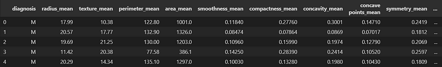

图 1.检查 DataFrame 的前 5 行

三、探索性数据分析

在本节中，我们将对 Breast Cancer Wisconsin 数据集进行探索性数据分析。这将涉及检查数据中是否存在任何 null 值并执行必要的数据预处理步骤。

3.1. 查找 null 值

为了确保数据的完整性，我们将首先调查是否存在任何 null 值。通过仔细检查数据集，我们可以识别缺失值并决定处理它们的适当策略。

df.isnull().sum()

通过在 DataFrame 上调用该函数，它会生成一个布尔掩码，其中表示 null 值并指示非 null 值。然后，应用该函数计算每列的值总和，从而有效地给出每列的 null 值计数。isnull()TrueFalsesum()True

DataFrame 'df' 没有任何 null 值，确保数据集完整，并且不需要对缺失值进行任何进一步的处理或插补。

3.2. 数据预处理

在识别出任何 null 值后，我们将继续进行数据预处理。数据集中的 “诊断” 功能是分类的，需要将其转换为数字格式，以便与各种机器学习算法兼容。通过将其转换为数值，我们可以对特征执行数学和统计运算。

# Replace M with 1 and Begnin with 0 (else 0)
print("Malignant=1, Benign=0")
df["diagnosis"]= df["diagnosis"].map(lambda row: 1 if row=='M' else 0)
df.head()

提供的代码通过将 'M' 替换为 1 （对于恶性病例）和 'B' （良性病例） 来完成此转换。

3.3. 独特价值

为了深入了解数据集，我们将检查不同列中存在的唯一值。此步骤使我们能够了解每个特征中的不同类别或级别，并识别任何潜在的数据不一致。

print("The unique number of data values are")
df.nunique()

3.4. 两种类型（恶性、良性）之间的数据传播

我们将在 “诊断” 列中评估恶性和良性病例之间的数据分布。通过分析每种类型的数量或比例，我们可以了解类不平衡并确定是否需要任何进一步的步骤，例如数据平衡技术。

import seaborn as sns

diagnosis_counts = df["diagnosis"].value_counts()
mean_diagnosis = df["diagnosis"].mean()
total_data_points = len(df)

print("Total number of data points =", total_data_points)
print("Malignant (diagnosis = 1) = {:.2f}%".format(mean_diagnosis * 100))
print("Benign (diagnosis = 0) = {:.2f}%".format((1 - mean_diagnosis) * 100))

sns.countplot(data=df, x="diagnosis")
plt.ylabel("Number of data points")
plt.title("Malignant (1) vs Benign Data(0) points")
plt.show()

首先，使用 计算每个唯一诊断（恶性或良性）的值计数df["diagnosis"].value_counts()。这为每个诊断类别提供了数据点的数量。

“诊断”列的平均值使用计算df["diagnosis"].mean()，表示数据集中恶性病例的比例。

然后，生成计数图，用来sns.countplot()可视化每个诊断类别的数据点分布。

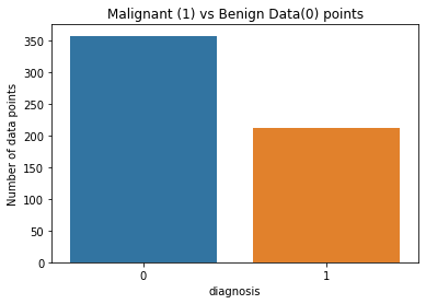
图 2.恶性 （1） vs 良性 （0）

3.5. 特征选择和降维

特征选择和降维是机器学习和数据分析中使用的两种常用技术。

要素选择涉及从原始要素集中选择相关要素的子集。它旨在消除不相关或冗余的特征，从而提高模型性能、减少过度拟合并增强可解释性。

另一方面，降维侧重于将原始的高维数据集转换为低维空间，同时保留最重要的信息。这有助于解决维度的诅咒，降低计算复杂性，并以更易于管理的方式可视化数据。

在实际项目中，可以根据特定目标和要求选择特征或降维。这两种技术都有助于提高模型性能和降低复杂性，但选择取决于数据集的性质和手头的问题。

3.5.1.特征选择

为了确定我们分析的相关特征，我们将使用相关矩阵。此矩阵提供每对特征之间线性关系的度量。通过检查相关性，我们可以识别高度相关的特征，并可能选择对我们的 Logistic 回归模型最有用的特征子集。

corr = df.corr()
corr[['diagnosis']].abs().sort_values(by='diagnosis', ascending=False)

变量 'corr' 存储使用 'df.corr（）' 计算的相关矩阵。此矩阵包含 DataFrame 中所有列对之间的相关系数。

通过使用 'corr[['diagnosis']]' 从相关矩阵中选择 'diagnosis' 列，并应用 'abs（）' 函数来计算相关性的绝对值，我们得到一个 DataFrame，其中包含 “diagnosis” 列和其他特征之间的绝对相关值。

'sort_values（）' 函数用于根据 “diagnosis” 列的绝对相关值对 DataFrame 进行降序排序。

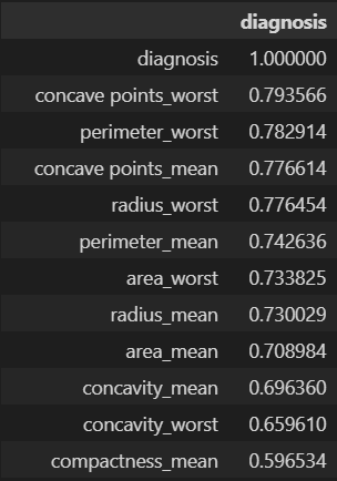
图 3.根据 “诊断” 列的绝对相关值降序排列

用于乳腺癌诊断的特征选择和相关矩阵可视化：

import pandas as pd
import seaborn as sns
import matplotlib.pyplot as plt
from sklearn.feature_selection import SelectKBest, f_regression, r_regression
import numpy as np

# Separate the features (X) and the target variable (y)
X = df.drop('diagnosis', axis=1) 
y = df['diagnosis']

# Perform feature selection 
'''
`SelectKBest` method is used for feature selection. 
It selects the top k features based on a scoring function
'''
selector = SelectKBest(score_func=f_regression, k=3) 
selected_features = selector.fit_transform(X, y)

# Get the indices of the selected features
selected_indices = selector.get_support(indices=True)

# Get the names of the selected features
selected_feature_names = X.columns[selected_indices]

# Print the selected feature names
print("Selected Features:")
print(selected_feature_names) # 'concave points_mean', 'perimeter_worst', 'concave points_worst'

# Create a DataFrame with the selected features
selected_df = X[selected_feature_names]

# Calculate the correlation matrix between selected features and target
correlation_matrix = selected_df.join(y).corr()
new_df = selected_df.join(y)

# mask the upper triangle of the correlation matrix, as it is redundant.
mask = np.triu(np.ones_like(correlation_matrix, dtype=bool))

# Create a heatmap to visualize the correlation matrix
plt.figure(figsize=(8, 6))
sns.heatmap(correlation_matrix, annot=True, cmap='coolwarm', mask=mask)
plt.title('Correlation Matrix between Selected Features and Target')
plt.show()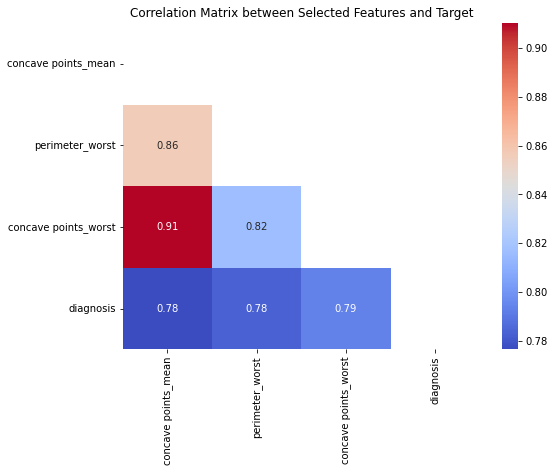

图 4.所选特征与目标变量之间的相关矩阵。

有关更多信息，请访问：

mask = np.triu(np.ones_like(correlation_matrix, dtype=bool))
print(mask)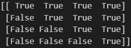

图 5.上三角矩阵

<span style="background-color:#f9f9f9"><span style="color:#242424">sns.heatmap(correlation_matrix, annot=<span style="color:#aa0d91">True</span>, cmap=<span style="color:#c41a16">'coolwarm'</span>, mask=mask)</span></span>

这是 seaborn 库绘制热图的文档 [链接]

mask：bool 数组或 DataFrame，可选

如果传递，则数据将不会显示在为 True 的单元格中。mask

这是我们在特征选择阶段后获得的新 DataFrame：

<span style="background-color:#f9f9f9"><span style="color:#242424">new_df.head()</span></span>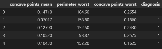

图 6.检查新 DataFrame 的前 5 行

3.5.2 降维 （PCA）

主成分分析 （PCA） 是一种降维技术，它将高维数据转换为低维空间，同时保留数据中最重要的模式和可变性。

<span style="background-color:#f9f9f9"><span style="color:#242424"><span style="color:#aa0d91">from</span> sklearn.preprocessing <span style="color:#aa0d91">import</span> StandardScaler
<span style="color:#aa0d91">from</span> sklearn.decomposition <span style="color:#aa0d91">import</span> PCA

X = df.drop([<span style="color:#c41a16">'diagnosis'</span>], axis=<span style="color:#1c00cf">1</span>)
y = df[<span style="color:#c41a16">'diagnosis'</span>]

X_scaled = StandardScaler().fit_transform(X)

pca = PCA(n_components=<span style="color:#1c00cf">2</span>)
X_pca_scaled = pca.fit_transform(X_scaled)

plt.figure(figsize=(<span style="color:#1c00cf">10</span>, <span style="color:#1c00cf">8</span>))
plt.scatter(X_pca_scaled[:, <span style="color:#1c00cf">0</span>], X_pca_scaled[:, <span style="color:#1c00cf">1</span>], c=df[<span style="color:#c41a16">'diagnosis'</span>], alpha=<span style="color:#1c00cf">0.7</span>, s=<span style="color:#1c00cf">30</span>, cmap=<span style="color:#c41a16">'plasma'</span>)
plt.xlabel(<span style="color:#c41a16">'PCA component 1'</span>)
plt.ylabel(<span style="color:#c41a16">'PCA component 2'</span>)
plt.title(<span style="color:#c41a16">'PCA projection of Breast Cancer Dataset'</span>)</span></span>

首先，特征 （X） 和目标变量 （y） 与 DataFrame 分开。为了准备 PCA 的数据，使用 scikit-learn 中的 StandardScaler 对特征进行缩放。'StandardScaler（）.fit_transform（X）' 将特征缩放为零均值和单位方差，从而产生X_scaled。

PCA 使用 'PCA（n_components=2）' 进行初始化，表示我们希望将数据投影到两个主组件上。'pca.fit_transform（X_scaled）' 线将 PCA 模型拟合到缩放特征并执行降维，从而产生包含投影数据的X_pca_scaled。

最后，创建一个散点图来可视化投影数据。散点图的 x 和 y 坐标分别取自 'X_pca_scaled[：， 0]' 和 'X_pca_scaled[：， 1]'。每个数据点的颜色由使用 'c=df['diagnosis']' 的 'diagnosis' 列确定，不同的颜色代表不同的诊断类别。设置透明度 （alpha）、标记大小 （s） 和颜色图 （cmap） 等其他参数以自定义绘图外观。

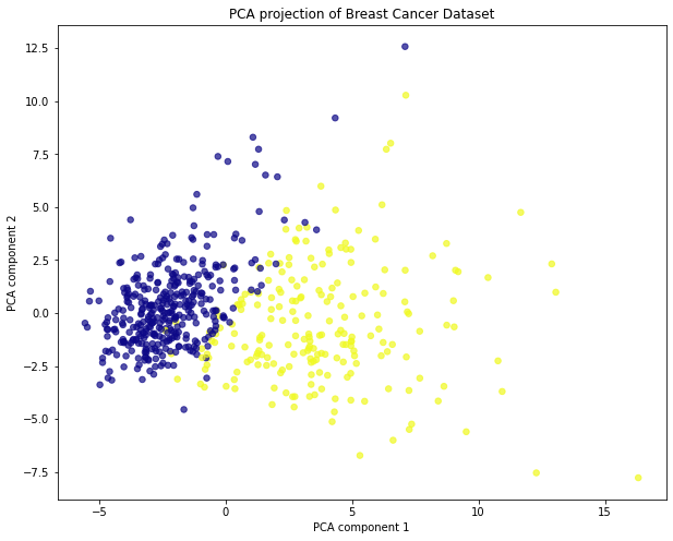
图 7.在二维空间中可视化数据

3.6. 选择数据的两个重要特征

corr计算DataFrame 的相关矩阵（ ） new_df，并根据“诊断”列的绝对相关值提取前三行。

corr = new_df.corr()
top_three_corr = corr[['diagnosis']].abs().sort_values(by='diagnosis', ascending=False).head(3)

print(top_three_corr)
'''
                      diagnosis
diagnosis              1.000000
concave points_worst   0.793566
perimeter_worst        0.782914
'''
new_df.head()

在删除 'concave points_mean' 功能之前：

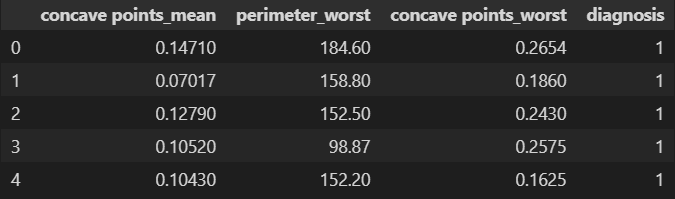
图 8.删除“凹points_mean”特征之前

删除引用特征：

new_df = new_df.drop(columns=['concave points_mean'], axis=1) 
new_df.head()

数据集的一些行：

图 9.删除“凹points_mean”特征后

3.7. 重命名列名称，以便它们可以进行编码

new_df.rename(columns={'concave points_worst': 'concave_points_worst'}, inplace=True)
new_df.head()

重命名后的 dataset 部分行：

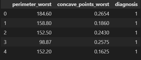
图 10.重命名后

四、数据规范化

数据归一化是机器学习中一个关键的预处理步骤，可确保数据集中的数值变量转换为通用比例。这有助于避免偏向于具有较大幅度的变量，并允许在不同变量之间进行公平比较。我们将探讨两种常见的数据规范化方法：

规范化和标准化。

4.1. 归一化

规范化（也称为最小-最大缩放）将数据重新缩放到介于 0 和 1 之间的范围。当数据分布未知或存在异常值时，此方法特别有用。以下是实现规范化的两种方法：

4.1.1 方法 1：自定义函数

def normalization(data, train_data):
    min_value = np.min(train_data, axis=0)
    max_value = np.max(train_data, axis=0)
    normalized_data = (data - min_value) / (max_value - min_value)
    return normalized_data

# Assuming train_data and test_data are the respective train and test sets
normalized_train = normalization(train_df, train_df)
normalized_test  = normalization(test_df, train_df)

在该函数中，使用 np.min 和 np.max 函数沿指定轴 （axis=0） 逐列计算最小值和最大值，从而确保独立获取每个特征的最小值和最大值。然后，通过减去最小值并除以每个特征的范围（最大值和最小值之间的差值）来规范化数据集数据。

为了将规范化应用于单独的训练集和测试集，该函数调用两次：一次用于训练集 （train_df），其中 train_df 作为数据和train_data传递，一次用于测试集 （test_df），其中 test_df作为数据传递，train_df作为 train_data 传递。这可确保根据从训练集计算的最小值和最大值执行规范化。

应用归一化之前训练数据集的 min、max 和 std：

print("Minimum values:")
print(train_df.min())
print()

print("Maximum values:")
print(train_df.max())
print()

print("Standard deviation:")
print(train_df.std())

图 11.应用规范化之前训练数据集的 Min、max 和 std

应用归一化后训练数据集的 min、max 和 std：

print("Minimum values:")
print(normalized_train.min())
print()

print("Maximum values:")
print(normalized_train.max())
print()

print("Standard deviation:")
print(normalized_train.std())

图 12.应用归一化后训练数据集的 Min、Max 和 std

4.1.2 方法 2：MinMaxScaler

或者，scikit-learn 提供了 'MinMaxScaler' 类，它简化了规范化过程。它通过减去最小值并除以范围 （maximum — minimum） 将数据缩放到指定范围（通常介于 0 和 1 之间）。当对多个数据集应用相同的缩放或在 scikit-learn 中使用管道时，此方法特别有用。

from sklearn.preprocessing import MinMaxScaler

scaler = MinMaxScaler()

# Fit the scaler on the train DataFrame
scaler.fit(train_df)

# Normalize the train DataFrame
normalized_train = scaler.transform(train_df)

# Normalize the test DataFrame using the fitted scaler
normalized_test = scaler.transform(test_df)

print(normalized_train.min(), normalized_train.max(), normalized_test.min(), normalized_test.max())
# (0.0, 1.0, -0.0207411926185756, 1.0)

'MinMaxScaler' 的 'fit_transform' 方法的输出类型是一个 numpy 数组。然后，将 fit 方法应用于 train_df 以计算规范化所需的最小值和最大值。随后，使用 transform 方法使用相同的 scaler 对象对训练和测试 DataFrame 进行规范化。这可确保根据从训练集获得的最小值和最大值，在两个数据集中一致地应用规范化。

4.2. 标准化

标准化（也称为 z 分数归一化）将数据转换为平均值 0 和标准差 1。标准化将数据集的特征转换为零均值和单位方差，使其遵循标准正态分布。它通常用于神经网络中，以确保输入特征具有一致的规模并促进学习过程。以下是标准化的两种方法：

4.2.1 方法 1：自定义函数

提供的代码片段演示了一个自定义函数 'standardization（x）'，该函数将变量（例如，DataFrame 的列）作为输入并返回标准化数据。它使用公式 '（x — x.mean（）） / x.std（）' 计算标准化值，其中 'x.mean（）' 和 'x.std（）' 分别表示变量的平均值和标准差。

def standardization(data, train_data):
    mean_value = np.mean(train_data, axis=0)
    std_value  = np.std(train_data, axis=0)
    standardized_data = (data - mean_value) / std_value
    return standardized_data

# standardized or simply normalized dataframe
standardized_train = standardization(train_df, train_df)
standardized_test  = standardization(test_df, train_df)

每个特征的最小和最大标准化值的可视化

import matplotlib.pyplot as plt

# Calculate the minimum and maximum values for each feature
min_values = standardized_train.min()
max_values = standardized_train.max()

# Create a bar plot
plt.figure(figsize=(8, 6))
plt.bar(min_values.index, min_values, label='Min')
plt.bar(max_values.index, max_values, label='Max')
plt.xlabel('Features')
plt.ylabel('Normalized Values')
plt.title('Minimum and Maximum Values for Each Feature')
plt.legend()
plt.show()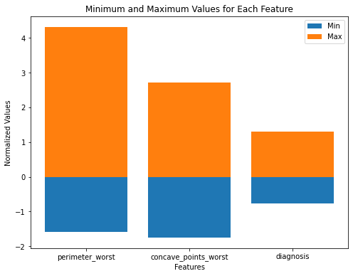

图 13.每个特征的最小值和最大值

4.2.2 方法 2：StandardScaler

或者，scikit-learn 提供了 'StandardScaler' 类，它简化了标准化过程。它通过减去平均值并除以标准差来标准化数据。

from sklearn.preprocessing import StandardScaler
scaler = StandardScaler()

standardized_train = scaler.fit_transform(train_df)
standardized_test =  scaler.transform(test_df)

五、使用 GridSearchCV 进行超参数调优和训练

GridSearchCV 是一种机器学习技术，可系统地为给定模型搜索超参数的最佳组合。

我想使用 Normalization method（归一化方法）：

new_df = new_df.drop(columns=['concave points_mean'], axis=1) 
train_df, test_df = train_test_split(new_df, test_size=0.2, random_state=42)

normalized_train = normalization(train_df, train_df)
normalized_test  = normalization(test_df, train_df)

# Extract features and target variable columns from normalized_train, and normalized_test
x_train = normalized_train.drop(['diagnosis'], axis=1).values
y_train = normalized_train['diagnosis'].values

x_test = normalized_test.drop(['diagnosis'], axis=1).values
y_test = normalized_test['diagnosis'].values

print(x_train.shape, y_train.shape, x_test.shape, y_test.shape)
# (455, 2) (455,) (114, 2) (114,)

使用 GridSearchCV 对 Logistic 回归模型进行超参数优化的过程：

from sklearn.model_selection import GridSearchCV
from sklearn.linear_model import LogisticRegression

# Define the parameter grid
param_grid = {
    'C': [0.01, 0.1, 1, 2, 5],
    'solver': ['lbfgs', 'liblinear', 'newton-cg', 'sag', 'saga']
}

clf = LogisticRegression()
model = GridSearchCV(clf, param_grid)
model.fit(x_train, y_train)
best_clf = model.best_estimator_

print(best_clf) 
# LogisticRegression(C=5, solver='liblinear')

定义了一个参数网格 'param_grid'，它指定要为 Logistic Regression 模型的超参数探索的不同值。在此示例中，正在优化的超参数是 'C' （正则化强度的倒数） 和 'solver' （用于优化的算法）。参数网格中提供了 'C' 和 'solver' 的各种值。

'GridSearchCV' 对象对指定的参数网格执行详尽搜索，使用交叉验证评估模型的性能。

'fit（）' 方法触发网格搜索过程，其中针对网格中的每种超参数组合训练和评估模型。网格搜索完成后， 'model.best_estimator_' 返回最佳估计器，即具有超参数最佳组合的 Logistic 回归模型。这个最佳模型可以分配给 'best_clf' 以供进一步使用。

5.1 用于模型评估的分类报告

scikit-learn 库中的 classification_report 函数是评估分类模型性能的强大工具。它提供了分类任务中每个类的各种评估指标的全面摘要，包括精度、召回率、F1 分数和支持。

分类报告将真实标签 （Ground Truth） 和预测标签作为输入，并计算每个类的评估指标。

精度衡量的是正确预测的正实例占预测为正的所有实例的比例，而召回率衡量的是正确预测的正实例占所有实际正实例的比例。F1 分数是精确率和召回率的调和平均值，提供模型准确率的平衡度量。

支持指标表示 true 标签中属于每个类的实例数。它可以帮助识别不平衡的类或提供对数据分布的见解。

from sklearn.metrics import classification_report

y_pred = best_clf.predict(x_test)
report = classification_report(y_test, y_pred)

print("Classification Report:")
print(report)

图 14.分类报告

5.2 决策边界的可视化

该模块中的函数提供了一种可视化分类模型的决策边界的便捷方法。它有助于理解模型如何根据提供的功能来分离不同的类。plot_decision_regionsmlxtend.plotting

from mlxtend.plotting import plot_decision_regions

fig, ax = plt.subplots(figsize=(6, 6))
plot_decision_regions(x_train, y_train.astype(np.int_), clf=best_clf)

ax.set_xlabel("Feature 1")
ax.set_ylabel("Feature 2")
ax.set_title("Decision Boundary")
plt.show()

clf 参数设置为 best_clf，表示经过训练的分类器模型。这允许该函数使用经过训练的模型根据提供的特征数据绘制决策边界。

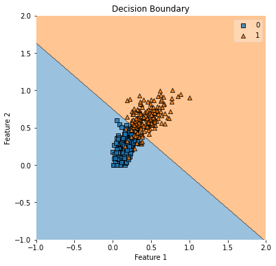
图 15.决策边界

六、结论

在第 14 天，我们讨论了为分类任务实施 Logistic 回归，并描述了所涉及的所有步骤。我们专注于数据准备、模型训练、评估和可视化。在我即将发布的博文。