关于粒子滤波的解析

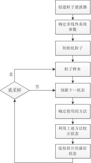
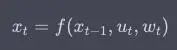
粒子滤波流程

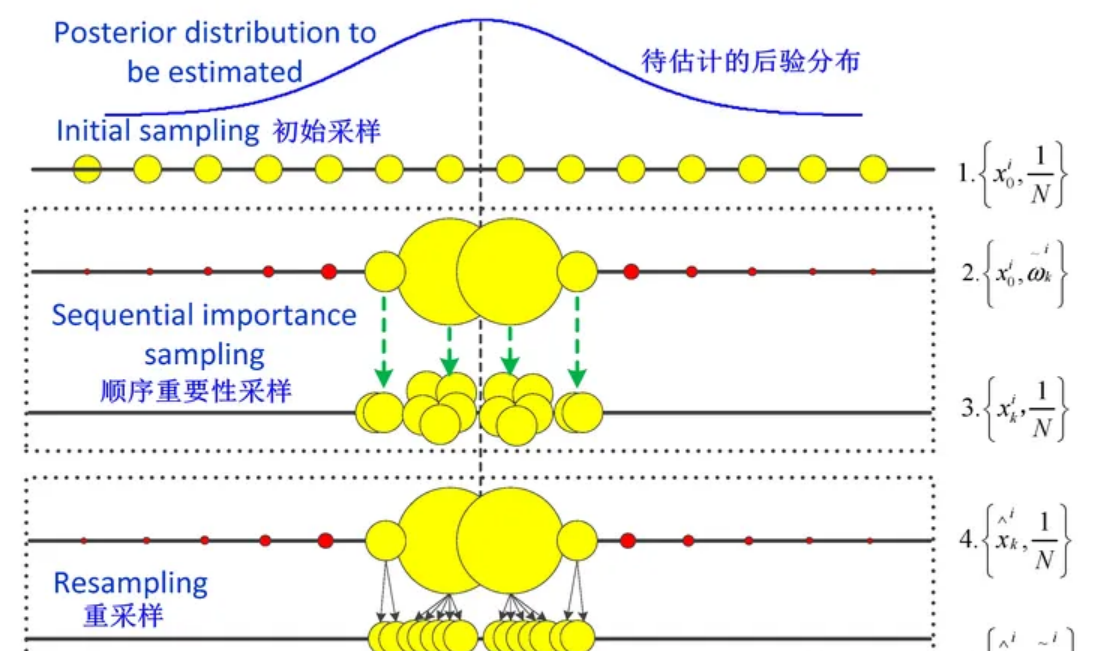
基本原理：随机选取预测域的 N NN 个点，称为粒子。以此计算出预测值，并算出在测量域的概率，即权重，加权平均就是最优估计。之后按权重比例，重采样，进行下次迭代。

初始状态：用大量粒子模拟X（t），粒子在空间内均匀分布；
预测阶段：根据状态转移方程，每一个粒子得到一个预测粒子；
校正阶段：对预测粒子进行评价，越接近于真实状态的粒子，其权重越大；
重采样：根据粒子权重对粒子进行筛选，筛选过程中，既要大量保留权重大的粒子，又要有一小部分权重小的粒子；
滤波：将重采样后的粒子带入状态转移方程得到新的预测粒子，即步骤2。

1. 初始状态

我们假设 GPS 的位置及航向输出服从正态分布，因此在得到 GPS 的初始输出后，我们可以根据初始值（均值 μ）和 GPS 观测不确定度（标准差 σ）构造无人车的定位初始分布，并通过对初始分布进行随机采样完成粒子集的初始化。

/**
 * @brief Initialize the particle filter.
 *
 * @param x Initial x position [m] from GPS.
 * @param y Initial y position [m] from GPS.
 * @param theta Initial heading angle [rad] from GPS.
 * @param std_pos Array of dimension 3 [standard deviation of x [m],
 *   standard deviation of y [m], standard deviation of theta [rad]]
 */
void ParticleFilter::Init(const double &x, const double &y, const double &theta,
                          const double std_pos[])
{
    if (!IsInited())
    {
        // create normal distributions around the initial gps measurement values
        std::default_random_engine gen;
        std::normal_distribution<double> norm_dist_x(x, std_pos[0]);
        std::normal_distribution<double> norm_dist_y(y, std_pos[1]);
        std::normal_distribution<double> norm_dist_theta(theta, std_pos[2]);

        // initialize particles one by one
        for (size_t i = 0; i < n_p; ++i)
        {
            particles(0, i) = norm_dist_x(gen);
            particles(1, i) = norm_dist_y(gen);
            particles(2, i) = norm_dist_theta(gen);
        }

        // initialize weights to 1 / n_p
        weights_nonnormalized.fill(1 / n_p);
        weights_normalized.fill(1 / n_p);

        is_inited = true;
    }
}

有几点说明如下：

这里使用了 C++ 的随机数引擎 std::default_random_engine 和正态分布模板类 std::normal_distribution 实现了高斯随机数的生成
particles 是 3×np3×np 的粒子 Eigen 矩阵，npnp 表示粒子数目，我们在构造函数的初始值列表中将其初始化为了 10001000，矩阵的每一列表示一个粒子的状态，矩阵的第 00、11、22 行分别表示粒子的横向位置 xx、纵向位置 yy 和航向角 thetatheta
weights_nonnormalized 和 weights_normalized 分别表示未归一化和归一化的重要性权重，数据类型都是 np×1np×1 的 Eigen 向量。很多粒子滤波教程中使用同一个变量存放未归一化和归一化的重要性权重，这样也是可以的，这里我们的目的是使代码逻辑更加清晰。

2. 预测阶段

根据机器人的车轮运动速度或者里程对粒子进行状态转移，即将粒子的信息带入机器人的运动模型中，加入控制噪声并产生新的粒子。

在预测步中，我们需要根据无人车的运动模型、车速、航向角速率、相邻两帧的时间间隔等将上一步的粒子集向当前时刻进行预测。

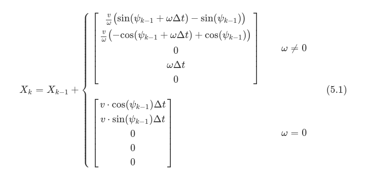
式 (5.1) 中，ωω 即自车的航向角速率。CTRV 是 CV 的一般形式，当 ω=0ω=0 时，CTRV 退化为 CV。

/**
 * @brief Predict new state of particle according to the system motion model.
 *
 * @param velocity Velocity of car [m/s]
 * @param yaw_rate Yaw rate of car [rad/s]
 * @param delta_t delta time between last timestamp and current timestamp [s]
 * @param std_pos Array of dimension 3 [standard deviation of x [m],
 *   standard deviation of y [m], standard deviation of yaw [rad]]
 */
void ParticleFilter::Predict(const double &velocity, const double &yaw_rate,
                             const double &delta_t, const double std_pos[])
{
    if (!IsInited())
        return;

    // create process noise's normal distributions of which the mean is zero
    std::default_random_engine gen;
    std::normal_distribution<double> norm_dist_x(0, std_pos[0]);
    std::normal_distribution<double> norm_dist_y(0, std_pos[1]);
    std::normal_distribution<double> norm_dist_theta(0, std_pos[2]);

    // predict state of particles one by one
    for (size_t i = 0; i < n_p; ++i)
    {
        double theta_last = particles(2, i);

        Eigen::Vector3d state_trans_item_motion;
        Eigen::Vector3d state_trans_item_noise;

        state_trans_item_noise << norm_dist_x(gen), norm_dist_y(gen), norm_dist_theta(gen);

        if (std::fabs(yaw_rate) > 0.001) // CTRV model
        {
            state_trans_item_motion << velocity / yaw_rate * (sin(theta_last + yaw_rate * delta_t) - sin(theta_last)),
                velocity / yaw_rate * (-cos(theta_last + yaw_rate * delta_t) + cos(theta_last)),
                yaw_rate * delta_t;
        }
        else // approximate CV model
        {
            state_trans_item_motion << velocity * cos(theta_last) * delta_t,
                velocity * sin(theta_last) * delta_t,
                yaw_rate * delta_t;
        }

        // predict new state of the ith particle
        particles.col(i) = particles.col(i) + state_trans_item_motion + state_trans_item_noise;

        // normalize theta
        NormalizeAngle(particles(2, i));
    }
}

状态转移过程中的过程噪声我们假设为零均值的高斯白噪声。很明显预测步只改变了每个粒子的状态，未改变粒子的权重。每个粒子的预测航向角我们都做了 [−π,π][−π,π] 的归一化处理，后面在计算系统最终的加权状态估计时不需要重复处理。

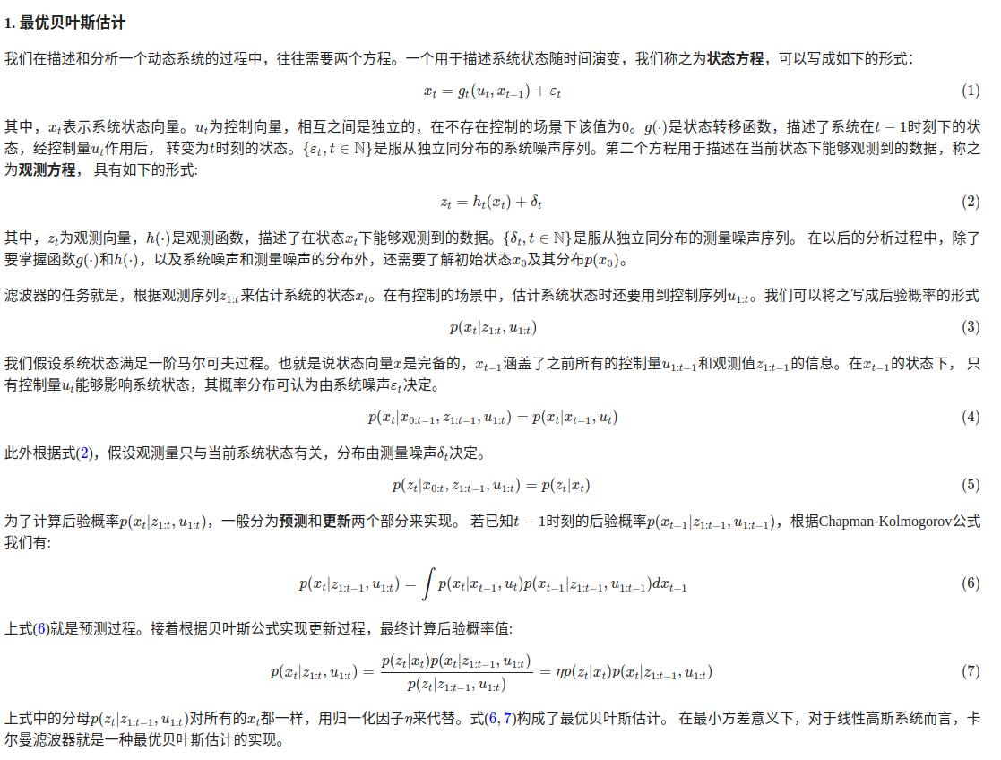
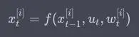
在粒子滤波中xtxt是在时刻tt的状态，utut是时刻tt的控制输入，wtwt是过程噪声，表示系统模型中的不确定性

3. 校正阶段

这里面其实涉及到几个步骤，其实主要起到的作用是更新+粒子权重更新的部分。

更新步的目的是根据最新的路标观测结果（自车局部坐标系下的横纵向相对位置），更新预测步后每个粒子的重要性权重。更新步主要由以下四个子步骤组成，需要对粒子集中的每个粒子依次执行以下步骤，我们结合代码进行阐述。

步骤 (1)：坐标变换

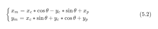
无人车实时观测到的路标结果基于自车局部坐标系，我们将其转换到地图的全局坐标系，关于坐标系变换推导并不复杂，可见参考 34。假设当前时刻自车观测到某个路标 lmrk(xc,yc)lmrk(xc,yc)，下角标 cc 表示自车坐标系，该路标对应于地图坐标系中的位置为 lmrk(xm,ym)lmrk(xm,ym)，下角标 mm 表示地图坐标系。对于粒子 p(xp,yp,θp)p(xp,yp,θp)，下角标 pp 表示粒子，我们直接给出从 lmrk(xc,yc)lmrk(xc,yc) 到 lmrk(xm,ym)lmrk(xm,ym) 的坐标变换方程。

/**
 * @brief Transform observed landmarks from local ego vehicle coordinate to
 *   global map coordinate.
 *
 * @param lmrks_obs Observed landmarks in ego vehicle coordinate.
 * @param particle Single particle with state of [x, y, theta]
 * @param lmrks_trans2map Observed landmarks transformed from local ego vehicle
 *   coordinate to global map coordinate.
 */
void ParticleFilter::TransLandmarksFromVehicle2Map(const std::vector<LandMark_Obs> &lmrks_obs,
                                                   const Eigen::Vector3d &particle,
                                                   std::vector<LandMark_Map> &lmrks_trans2map)
{
    for (size_t i = 0; i < lmrks_obs.size(); ++i)
    {
        lmrks_trans2map[i].x = lmrks_obs[i].x * cos(particle(2)) -
                               lmrks_obs[i].y * sin(particle(2)) + particle(0);

        lmrks_trans2map[i].y = lmrks_obs[i].x * sin(particle(2)) +
                               lmrks_obs[i].y * cos(particle(2)) + particle(1);
    }
}

这一部分其实就是构建观测模型，其描述了如何将系统状态映射到观测值。通常，这可以用一个非线性函数来表示。其中，ztzt是在时刻tt的观测值，vtvt是观测噪声，表示观测模型中的不确定性。如果是深度学习给到的分割结果，这里可以直接用输入数据（如上）

步骤 (2)：查找传感器感知范围内的地图路标

传感器的实际感知范围是有限的，我们需要找到每个粒子对应的传感器感知范围内的地图路标。

/**
 * @brief Find map landmarks within the sensor measuremet range.
 *
 * @param lmrks_map All map landmarks.
 * @param particle Single particle with state of [x, y, theta]
 * @param snsr_range Sensor measuremet range.
 * @param lmrks_within_range Map landmarks within the sensor measuremet range.
 */
void ParticleFilter::FindMapLandmarksWithinSensorRange(const std::vector<LandMark_Map> &lmrks_map,
                                                       const Eigen::Vector3d &particle,
                                                       const double &snsr_range,
                                                       std::vector<LandMark_Map> &lmrks_within_range)
{
    static double distance_threshold_square = snsr_range * snsr_range;

    for (auto landmark : lmrks_map)
    {
        double distance_square = std::pow(particle(0) - landmark.x, 2) +
                                 std::pow(particle(1) - landmark.y, 2);

        if (distance_square <= distance_threshold_square)
            lmrks_within_range.push_back(landmark);
    }
}

步骤 (1) 和步骤 (2) 作为步骤 (3) 的输入，其顺序无关紧要。

步骤 (3)：数据关联

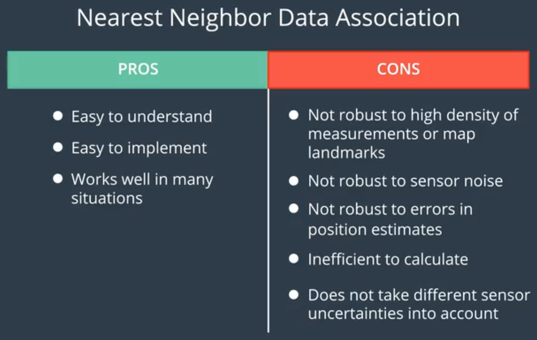
数据关联的目的是找到观测路标与实际地图路标的一一对应关系，步骤 (4) 中需要通过这个对应关系更新每个粒子的权重。这里我们使用一种最为简单的数据关联方法——最近邻（Nearest Neighbor，NN）数据关联，其核心思想很直观：对于两个待关联的数据集，数据间的欧氏距离越小，关联的概率越高。NN 数据关联方法的优缺点总结如下（图片出自 Udacity）。

![在这里插入图片描述](https://i-blog.csdnimg.cn/blog_migrate/5eda32fe41607c7bf83bee9a09809745.png)/**
 * @brief Associate observed landmarks which have been transformed to global
 *   map coordinate with map landmarks within the sensor measuremet range.
 *
 * @param lmrks_within_range Map landmarks within the sensor measuremet range.
 * @param lmrks_trans2map Observed landmarks transformed from local ego vehicle
 *   coordinate to global map coordinate.
 */
void ParticleFilter::DataAssociation(const std::vector<LandMark_Map> &lmrks_within_range,
                                     std::vector<LandMark_Map> &lmrks_trans2map)
{
    for (auto &landmark_trans2map : lmrks_trans2map)
    {
        double distance_min = std::numeric_limits<double>::max();

        for (auto &landmark_within_range : lmrks_within_range)
        {
            double distance_square = std::pow(landmark_trans2map.x - landmark_within_range.x, 2) +
                                     std::pow(landmark_trans2map.y - landmark_within_range.y, 2);

            if (distance_square < distance_min)
            {
                distance_min = distance_square;
                landmark_trans2map.id = landmark_within_range.id;
            }
        }
    }
}

在粒子滤波的预测步骤中，每个粒子根据状态传递模型进行状态的预测。这可以表示为.其中，utut是时刻tt的控制输入，wt[i]wt[i]表示第ii个粒子的过程噪声。

步骤 (4)：粒子权重更新

执行完关联步后，每个观测路标都对应一个地图路标，我们需要根据每个观测路标与地图路标的关联匹配程度来计算粒子的似然概率。这里我们假设对每个路标的观测都服从二元高斯分布，且相互独立，观测噪声也是高斯的，则每个观测路标的似然概率密度为

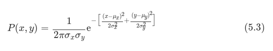
其中，xx 和 yy 分别表示观测路标转换到地图坐标系后的横向位置和纵向位置，μxμx 和 μyμy 分别表示观测路标关联上的地图路标的横向位置和纵向位置， σxσx 和 σyσy 表示路标观测的标准差。由于对每个路标的观测相互独立，粒子的总的似然概率密度为

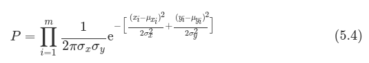
其中，mm 表示观测路标的数量。将每个观测路标转换到地图坐标系后的测量值代入式 (5.4) 便可得到粒子总的似然概率，结合粒子上一时刻的权重便可近似地序贯更新粒子当前时刻的权重（未归一化的）。下面我们给出权重更新部分的 C++ 实现。

/**
 * @brief For each observed landmark with an associated landmark, calculate
 *   its' weight contribution, and then multiply to particle's final weight.
 *
 * @param lmrks_trans2map Observed landmarks transformed from local ego vehicle
 *   coordinate to global map coordinate.
 * @param lmrks_map All map landmarks.
 * @param std_lmrks Array of dimension 2 [Landmark measurement uncertainty
 *   [x [m], y [m]]]
 * @param weight Non-normalized weight of particle.
 */
void ParticleFilter::UpdateWeight(const std::vector<LandMark_Map> &lmrks_trans2map,
                                  const std::vector<LandMark_Map> &lmrks_map,
                                  const double std_lmrks[],
                                  double &weight)
{
    double likelyhood_probability_particle = 1.0;
    double sigma_x = std_lmrks[0];
    double sigma_y = std_lmrks[1];

    for (auto &landmark_trans2map : lmrks_trans2map)
    {
        double x = landmark_trans2map.x;
        double y = landmark_trans2map.y;
        double ux = lmrks_map.at(landmark_trans2map.id - 1).x;
        double uy = lmrks_map.at(landmark_trans2map.id - 1).y;
        double exponent = -(std::pow(x - ux, 2) / (2 * std::pow(sigma_x, 2)) +
                            std::pow(y - uy, 2) / (2 * std::pow(sigma_y, 2)));
        double likelyhood_probability_landmark = 1.0 / (2 * M_PI * sigma_x * sigma_y) *
                                                 std::exp(exponent);
        likelyhood_probability_particle *= likelyhood_probability_landmark;
    }

    weight *= likelyhood_probability_particle;
}

下面是整个更新步的代码实现。

 * @brief
 *
 * @param lmrks_obs Observed landmarks in local ego vehicle coordinate.
 * @param snsr_range Sensor measuremet range.
 * @param lmrks_map All map landmarks.
 * @param std_lmrks Array of dimension 2 [Landmark measurement uncertainty
 *   [x [m], y [m]]]
 */
void ParticleFilter::Update(const std::vector<LandMark_Ego> &lmrks_obs,
                            const double &snsr_range,
                            const std::vector<LandMark_Map> &lmrks_map,
                            const double std_lmrks[])
{
    // process particles one by one
    for (size_t i = 0; i < n_p; ++i)
    {
        // step1: transform observed landmarks from local ego vehicle coordinate
        // to global map coordinate
        std::vector<LandMark_Map> landmarks_trans2map(lmrks_obs.size());
        TransLandmarksFromVehicle2Map(lmrks_obs, particles.col(i), landmarks_trans2map);

        // step2: find map landmarks within the sensor measuremet range
        std::vector<LandMark_Map> landmarks_within_sensor_range;
        FindMapLandmarksWithinSensorRange(lmrks_map, particles.col(i), snsr_range,
                                          landmarks_within_sensor_range);

        // step3: associate observed landmarks which have been transformed to
        // global map coordinate with map landmarks within the sensor measuremet
        // range
        DataAssociation(landmarks_within_sensor_range, landmarks_trans2map);

        // step4: for each observed landmark with an associated landmark, calculate
        // its' weight contribution, and then multiply to particle's final weight
        UpdateWeight(landmarks_trans2map, lmrks_map, std_lmrks, weights_nonnormalized(i));
    }
}

在权重更新步骤中，我们计算每个粒子的权重，以反映其与观测值的拟合程度。通常，权重的计算基于观测模型的似然度。其中，ztzt是在时刻tt的观测值，vtvt表示观测噪声。

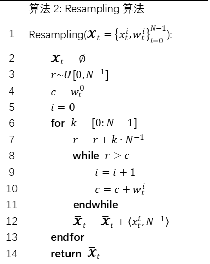
4 . 粒子权重归一化和重采样

在重采样步骤中，根据粒子的权重重新选择粒子，以便更有可能保留高权重的粒子，减少低权重的粒子。这有助于确保粒子集合更好地逼近真实的后验分布。主要分为两个步骤粒子权重归一化和重采样

4.1 粒子权重归一化

完成粒子非归一化权重的更新后，我们需要计算粒子新的归一化的权重，作为后面重采样步骤的输入。

/**
 * @brief Normalize the weights of particles.
 *
 * @param w_nonnormalized Weights to be normalized.
 * @param w_normalized Weights which have been normalized.
 */
inline void NormalizeWeights(const Eigen::VectorXd &w_nonnormalized,
                             Eigen::VectorXd &w_normalized)
{
    w_normalized = w_nonnormalized / w_nonnormalized.sum();
}

4.2 重采样

完成粒子权重归一化后，我们需要对粒子集进行重采样。对于重采样步骤，大多数基于 Udacity 工程框架的开源项目使用了 C++ 标准库中的离散分布模板类 std::discrete_distribution ，这里我们“舍近求远”，手工实现 3.3.1 节中介绍的四种重采样算法，以加深对重采样的理解，随机数的生成我们通过模板类 std::uniform_real_distribution 实现。

多项式重采样

/**
 * @brief Multinomial resampling method.
 *
 * @param particles_ori Particles before resampling.
 * @param weights_ori_norm Normalized weights before resampling.
 * @param particles_resampled Particles after resampling.
 * @param weights_resampled Weights after resampling.
 * @param N_r Number of particles to resample.
 */
void ParticleFilter::MultinomialResampling(const Eigen::MatrixXd &particles_ori,
                                           const Eigen::VectorXd &weights_ori_norm,
                                           Eigen::MatrixXd &particles_resampled,
                                           Eigen::VectorXd &weights_resampled,
                                           uint32_t N_r)
{
    uint32_t N = weights_ori_norm.size();
    uint32_t left, right, middle;

    Eigen::VectorXd weights_cum_sum = CalcWeightsCumSum(weights_ori_norm);

    for (size_t j = N - N_r; j < N; ++j)
    {
        // produces random values u, uniformly distributed on the interval [0.0, 1.0)
        std::random_device rd;
        std::mt19937 gen(rd());
        std::uniform_real_distribution<> uniform_dist(0.0, 1.0);
        double u = uniform_dist(gen);

        // select the resampled particle using binary search
        left = 0;
        right = N - 1;
        while (left < right)
        {
            middle = std::floor((left + right) / 2);
            if (u > weights_cum_sum(middle))
                left = middle + 1;
            else
                right = middle;
        }

        particles_resampled(j) = particles_ori(right);
        weights_resampled(j) = 1 / N;
    }
}

分层重采样

/**
 * @brief Stratified resampling method.
 *
 * @param particles_ori Particles before resampling.
 * @param weights_ori_norm Normalized weights before resampling.
 * @param particles_resampled Particles after resampling.
 * @param weights_resampled Weights after resampling.
 * @param N_r Number of particles to resample.
 */
void ParticleFilter::StratifiedResampling(const Eigen::MatrixXd &particles_ori,
                                          const Eigen::VectorXd &weights_ori_norm,
                                          Eigen::MatrixXd &particles_resampled,
                                          Eigen::VectorXd &weights_resampled,
                                          uint32_t N_r)
{
    uint32_t N = weights_ori_norm.size();

    Eigen::VectorXd weights_cum_sum = CalcWeightsCumSum(weights_ori_norm);

    uint32_t i = 0;

    for (size_t j = N - N_r; j < N; ++j)
    {
        // produces random values u0, uniformly distributed on the interval [0.0, 1.0 / N_r)
        // then calculate u = u0 + (j - (N - N_r)) / N_r
        std::random_device rd;
        std::mt19937 gen(rd());
        std::uniform_real_distribution<> uniform_dist(0.0, 1 / N_r);
        double u0 = uniform_dist(gen);
        double u = u0 + (j - (N - N_r)) / N_r;

        // select the resampled particle
        while (weights_cum_sum(i) < u)
            ++i;

        particles_resampled(j) = particles_ori(i);
        weights_resampled(j) = 1 / N;
    }
}

系统重采样

/**
 * @brief Systematic resampling method.
 *
 * @param particles_ori Particles before resampling.
 * @param weights_ori_norm Normalized weights before resampling.
 * @param particles_resampled Particles after resampling.
 * @param weights_resampled Weights after resampling.
 * @param N_r Number of particles to resample.
 */
void ParticleFilter::SystematicResampling(const Eigen::MatrixXd &particles_ori,
                                          const Eigen::VectorXd &weights_ori_norm,
                                          Eigen::MatrixXd &particles_resampled,
                                          Eigen::VectorXd &weights_resampled,
                                          uint32_t N_r)
{
    uint32_t N = weights_ori_norm.size();

    Eigen::VectorXd weights_cum_sum = CalcWeightsCumSum(weights_ori_norm);

    uint32_t i = 0;

    // produces random values u0, uniformly distributed on the interval [0.0, 1.0 / N_r)
    std::random_device rd;
    std::mt19937 gen(rd());
    std::uniform_real_distribution<> uniform_dist(0.0, 1 / N_r);
    double u0 = uniform_dist(gen);

    for (size_t j = N - N_r; j < N; ++j)
    {
        // calculate u = u0 + (j - (N - N_r)) / N_r
        double u = u0 + (j - (N - N_r)) / N_r;

        // select the resampled particle
        while (weights_cum_sum(i) < u)
            ++i;

        particles_resampled(j) = particles_ori(i);
        weights_resampled(j) = 1 / N;
    }
}

残差重采样

/**
 * @brief Residual resampling method.
 *
 * @param particles_ori Particles before resampling.
 * @param weights_ori_norm Normalized weights before resampling.
 * @param particles_resampled Particles after resampling.
 * @param weights_resampled Weights after resampling.
 */
void ParticleFilter::ResidualResampling(const Eigen::MatrixXd &particles_ori,
                                        const Eigen::VectorXd &weights_ori_norm,
                                        Eigen::MatrixXd &particles_resampled,
                                        Eigen::VectorXd &weights_resampled)
{
    uint32_t N = weights_ori_norm.size();
    uint32_t j = 0;
    Eigen::VectorXi N_k1(N);

    // step1: deterministic copy sampling
    for (size_t i = 0; i < N; ++i)
    {
        N_k1(i) = std::floor(N * weights_ori_norm(i));

        for (size_t m = 0; m < N_k1(i); ++m)
        {
            particles_resampled(j) = particles_ori(i);
            weights_resampled(j) = 1 / N;
            ++j;
        }
    }

    // step2: residual random sampling
    uint32_t N_k2 = N - j;
    Eigen::VectorXd weights_residual_norm = (N * weights_ori_norm - N_k1) / N_k2;
    MultinomialResampling(particles_ori, weights_residual_norm, particles_resampled,
                          weights_resampled, N_k2);
}

5. 滤波状态估计

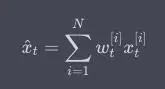
完成重采样后，我们将所有的重采样粒子及其对应的重采样权重（1NN1）进行加权求和，便可得到系统最终的状态估计结果，即每个时刻无人车的位置、航向估计。

/**
 * @brief Estimate the final state of system by combing all particles.
 *
 * @param particles_resampled Particles after resampling.
 * @param weights_resampled Weights after resampling.
 * @param particles_ori Particles before resampling.
 * @param weights_ori_norm Normalized weights before resampling.
 * @param weights_ori Non-normalized weights before resampling.
 * @return Eigen::Vector3d The final estimated state of system.
 */
inline Eigen::Vector3d EstimateState(const Eigen::MatrixXd &particles_resampled,
                                     const Eigen::VectorXd &weights_resampled,
                                     Eigen::MatrixXd &particles_ori,
                                     Eigen::VectorXd &weights_ori_norm,
                                     Eigen::VectorXd &weights_ori)
{
    particles_ori = particles_resampled;
    weights_ori = weights_resampled;
    weights_ori_norm = weights_resampled;

    return particles_ori * weights_ori_norm;
}

最后，在状态估计步骤中，我们使用重采样后的粒子集合来计算状态的估计值。通常，估计可以表示为对粒子状态乘以相应权重的加权平均：